Probabilistic Melody Modeling
One of the most challenging tasks in building a beautiful piece of music lies in composing a well-received melody. But what makes a good melody? Or, in a more generative sense:
How can we generate a beautiful melody algorithmically?
Because a melody can be seen as a series of numbers, it is not surprising that this question is a rather old one. Long before the digital computer, composers tried to constrain themselves by strategies and rules to limit the space of possibilities. In my opinion, limitations are necessary for a creative process.
If we can create everything, we become unable to express anything.
Therefore, it makes sense to invent rules that limit our possibilities.
Surprise, Repetition and Expectation
One general consensus is that a good melody balances repetition and surprise. If we can no longer recognize a structure and cannot guess what might be the following note or chord, a melody begins to lose its ability to transport emotion; it can no longer tell a story. On the other hand, if the melody is too repetitive, we get bored because the guessing game is too simple.
Computer scientists know the relation between surprise and repetition very well. We call it entropy. I will discuss the formal definition of entropy in another article. For now, it is only vital that entropy is a measure of surprise in a message we receive (on a purely syntactical level). For example, the result heads of a coin toss of a fair coin is less surprising than the result heads of a coin that is biassed towards tails. If an event is unlikely, its appearance is surprising.
Concerning the coin toss example, a message consists of multiple coin toss results. Let’s say 0 represents heads, and 1 represents tails, then 010111 is a message. The entropy of a message is a measure of how surprising it is to appear in a system that generates messages. To compute the entropy of a system that generates messages of length $n$, we sum up all surprises of each possible message of length $n$ and divide the result by $n$. For example, for an unbiased coin, the messages 00, 01, 10, and 11 appear with equal probability, i.e., $1/4$. The entropy is
\begin{equation} \frac{-1/4 \cdot \log_2(1/4) \cdot 4}{4} = 1. \end{equation}
Let us compare this with a biased coin. So let us assume heads has probability $0.2$ and tails has probability $0.8$, then we have 00 with probability $0.2^2 = 0.04$, 01 and 10 with probability $0.2 \cdot 0.8 = 0.16$ and 11 with probability $0.8^2 = 0.64$. Consequently, we get
\begin{equation} \frac{-0.04 \cdot \log_2(0.04) -2 \cdot 0.16 \cdot \log_2(0.16) -0.64 \cdot \log_2(0.64)}{4} \approx 0.361. \end{equation}
One could say the second system is less surprising to observers; it is more repetitive. In information theory we say the second system generates less information, but the term information can be misleading because it has nothing to do with meaning. From this perspective, a bunch of random numbers is regarded as more informative than a book.
In 1948 Claude E. Shannon established A mathematical theory of information (Shannon, 1948). He established the term entropy as a measurement of information, but he emphasized its limitation to syntax:
Frequently, the messages have meaning; that is, they refer to or are correlated according to some system with certain physical or conceptual entities. These semantic aspects of communication are irrelevant to the engineering problem. The significant aspect is that the actual message is one selected from a set of possible messages. The system must be designed to operate for each possible selection, not just the one which will actually be chosen since this is unknown at the time of design. – Claude E. Shannon
Even though there is no direct relation between entropy / information and meaning, we can look at extreme cases. If the entropy is very high (chaos) or very low (no information), a message will likely be meaningless to us, even subjectively. If we interpret a series of notes as a musical message, this statement is true in a musical context. We can apply the frequentist perspective, i.e., interpret frequencies as probabilities. We could generate melodies randomly and pick those within a predefined entropy range to achieve a balance between surprise and repetition.
However, a far better measurement, with regards to music, is expectation in the time domain. Music indicates no concepts or objects but more music that is about to happen. Good music has to make sense. It can disrupt our model of the world but not too much, such that we can adapt our model. I refer to our model of the world as interpretation; we are all interpreters of our perceptions. In that sense, actively listening to music is a process of constant model adaptation; the interpretation changes if something can not be interpreted.
Maybe that is, in fact, the key to the definition of meaning in general. Some observation is meaningful if it makes sense, and it can only make sense if we are able to adapt our interpretation in such a way that our observation fits in. This adaptation disrupts us; it changes our predictions. If it is marginal, we avoid losing ourselves because most predictions are still valid. But if the disruption attacks the very essence of our constructed self, we can no longer make sense of it.
Embodied musical meaning is […] a product of expectation – Leonard Meyer (1959)
Musical cognition implies the simultaneous recognition of a permanent and changeable element (Loy, 2006); it requires perception and memory. We have to perceive and compare pitches at the same time. The expectation is realized for different scales but has to be local and context-sensitive within the computation. Therefore, it is not only the distribution of notes (or rhythmic elements) within a composition but the distribution of their relation, i.e., their conditional probability distribution.
From Serialism to Probability
One way to generate melodies is to use the mathematical branch of combinatorics. The idea is simple: define a bunch of chords or notes that fit together and use permutation, rotation, and other combinatoric tricks to combine them. This kind of composition method belongs to serialism. However, the problem with this approach is that each note appears with equal probability; it neglects the importance of distributions and context. Consequently, the melody’s entropy is high.
In the 20th century, this approach was criticized by, for example, Iannis Xenakis.
Linear polyphony destroys itself by its very complexity; what one hears is, in reality, nothing but a mass of notes in various registers. The enormous complexity prevents the audience from following the intertwining of the lines and has as its macroscopic effect an irrational and fortuitous dispersion of sounds over the whole extent of the sonic spectrum. There is consequently a contradiction between polyphonic linear systems and the heard result, which is surface or mass. – Iannis Xenakis (1955)
He and his fellow critics pointed at the lack of orientation. They argued that generating melodies by a series of notes that can appear equally likely, results in a sound without structure, thus a disengaged audience.
Influenced by the development in quantum physics at that time (1971) and the isomorphism between the Fourier series and quantum analysis of sound, Xenakis believed that the listener experiences only the statistical aspects of serial music. Consequently, he reasoned that composers should switch from serial techniques to probability. And as a logical step, he drew his attention to the computer.
With the aid of electronic computers, the composer becomes a sort of pilot: he presses the buttons, introduces coordinates, and supervises the controls of a cosmic vessel sailing in the space of sound across sonic constellations and galaxies that he could formerly glimpse only as a distant dream. – Iannis Xenakis (1971)
Markov Chains
Let us now dive into a first attempt to generate melodies that incorporates probability and, as a consequence, expectation. The mathematical tool is called Markov chain.
A first-order Markov chain is a deterministic finite automaton where for each state transition, we assign a probability such that the sum of probability of all exiting transitions of each state sum up to 1.0. In other words, a first-order Markov chain is a directed graph where each node represents a state. We start with an initial node and traverse the graph probabilistically to generate an output.
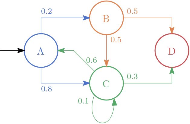
In the following figure, you can see a first-order Markov chain.
One starts in the state A and transits to B with a probability of 0.2 or C with a probability of 0.8.
D is a final state.
A possible series of states would be: ABCCACD
Given state A, the probability of moving to state B is equal to 0.2.
In other words
\begin{equation} P(X_{k+1} = B\ |\ X_{k} = A) = 0.2. \end{equation}
A first-order Markov chain only considers one predecessor, i.e., only the most local part of the context. A \(n\)-order Markov chain does consider \(n\) predecessors. In general, we define
\begin{equation} P(X_{k+1} = x\ |\ X_{k} = x_k, X_{k-1} = x_{k-1}, \ldots X_{k-n} = x_{k-n}) = p. \end{equation}
The visualization of such a chain is a little bit more complicated.
Music Generation
We can generate a composition by traversing the graph if we represent our notes by states of a Markov chain. If we increase the order of the chain, i.e. \(n\), the entropy decreases for small \(n\).
Until now, I only tried to use and generate a first-order Markov chain.
Even though I am not that familiar with Ruby, I used Sonic Pi for this task such that I can play around with it directly within the IDE of Sonic Pi.
I decided to define a note as a tuple (list) consisting of the pitch and the length of the note.
[:c4, 1.0/8] # a c of length 1/8 beat
Instead of a graph, I use a transition matrix \(P \in \mathbb{R}^{m \times m}\) where \(m\) is the number of states/notes. Let \(Q = \{q_1, \ldots, q_m\}\) be the set of states/notes. The entry of row \(i\) and column \(j\), i.e., \(p_{ij}\) is the probability of going from state \(q_i\) to state \(q_j\).
After constructing the matrix \(P\), the states \(Q\) and picking a start (state number), the following function generates a random melody of length n.
define :gen_mmelody do |n, matrix, start, states|
  #
  # Generates a random melody of length n based on a transition matrix
  # and an initial statenumber (start).
  #
  notes = [states[start]]
  from = start
  (n-1).times do
    p = rrand(0, 1)
    sum = 0
    to_row = matrix[from]
    to = 0
    while sum < p
      sum += to_row[to]
      to += 1
    end
    notes += [states[to-1]]
    from = to-1
  end
  return notes
end
For each note, we roll the dice. Let’s say \(p \in [0;1]\) is our result. And \(q_i\) is our current state. Then we compute \(j\) such that
\begin{equation} \sum\limits_{k=1}^{j-1} p_{ij} < p \leq \sum\limits_{k=1}^{j} p_{ij}. \end{equation}
Note that the code is not optimized in any way.
Learning a Markov Chain
Instead of generating a melody or rhythm given a Markov chain, we can do the reverse. Given a melody, we can learn the Markov chain that most likely would generate the given melody. By doing so, we can then use the learned chain to generate music in a similar style.
Let us use the same transition matrix \(P \in \mathbb{R}^{m \times m}\) where \(m\) is the number of states/notes. Let \(Q = \{q_1, \ldots, q_m\}\) be the set of states/notes. The entry of row \(i\) and column \(j\), i.e., \(p_{ij}\) is the probability of going from state \(q_i\) to state \(q_j\).
Furthermore, let us define our set of all possible melodies \(M \subseteq Q^n\) of length \(n\). Then a specific melody \(\mathbf{m} = (m_1, \ldots, m_n) \in M\) is a tuple (list) of notes:
notes = [[:g4, 1.0/8], [:g4, 1.0/8], [:a4, 1.0/4], [:g4, 1.0/4], ... ]
We can compute the most likely \(P\) by computing each entry of it where \(p_{ij}\) is equal to
\begin{equation} p_{ij} = \frac{n_{ij}}{n_i} \end{equation}
where \(n_{ij}\) is the number of transitions from \(q_i\) to \(q_j\) within \(\mathbf{m}\) and \(n_i\) is the number of transition starting at \(q_i\).
Given \(Q\) states and \(\mathbf{m}\) notes the following function computes \(P\) matrix.
define :gen_markov_matrix do |states, notes|
  #
  # Generates the transition matrix based on the set of notes (states)
  # and a given piece of music (notes).
  #
  matrix = Array.new(states.length, 0)

  for i in 0..(states.length-1)
    matrix[i] = Array.new(states.length, 0)
  end

  # (1) count transitions
  for i in 0..(notes.length-1)
    for from in 0..(states.length-1)
      for to in 0..(states.length-1)
        if notes[i] == states[from] && notes[i+1] == states[to]
          matrix[from][to] += 1.0
        end
      end
    end
  end
  # (2) normalize
  for from in 0..(states.length-1)
    s = matrix[from].sum
    for to in 0..(states.length-1)
      matrix[from][to] /= s
    end
  end
  print_matrix matrix, states
  return matrix
end
Of course, we can easily compute \(Q\) states from \(\mathbf{m}\) notes.
Finally, the following function takes a number n and a melody notes and generates a random melody of length n by learning \(P\) based on notes.
define :markov_melody do |n, notes|
  states = notes.uniq
  matrix = gen_markov_matrix(states.ring, notes.ring)
  return gen_mmelody(n, matrix, rand_i(states.length-1), states)
end
Example
I use the beginning of Bach’s Minuet in G.
I generate two melodies (by using a different seed) consisting of 34 notes:
Of course, this sound is not that musical. The rhythm is all over the place, but we recognize the original composition. Furthermore, no one said we have to stop there. We can continue to generate until we find something that sticks. Furthermore, this example is straightforward because I only use the beginning of one piece. Instead, we could use multiple compositions that fit together.
Code
This project was part of our workshop AI and Creativity to show a basic example of using artificial intelligence to generate music.
You can find the full example containing two different melodies on my GitHub page. The code includes some additional functions, e.g., a function that prints out the Markov matrix in a readable format.
References
- Shannon, C. E. (1948). A mathematical theory of communication. Bell Syst. Tech. J., 27(3), 379–423.
- Loy, G. (2006). Musimathics: The Mathematical Foundations of Music (Vol. 1). MIT Press.