Musical Interrogation IV - Transformer
This article is Part 4 in a 4-Part Series.
- Part 1 - Musical Interrogation I - Intro
- Part 2 - Musical Interrogation II - MC and FFN
- Part 3 - Musical Interrogation III - LSTM
- Part 4 - Musical Interrogation IV - Transformer
Recurrent models trained in practice are effectively feed-forward. This could happen either because truncated backpropagation through time cannot learn patterns significantly longer than k steps, or, more provocatively, because models trainable by gradient descent cannot have long-term memory. – John Miller
This time in the series we use the most famous model architecture for generative purposes: the transformer (Vaswani et al., 2017). Transformers were initially targeted at natural language processing (NLP) problems, where the network input is a series of high-dimensional embeddings representing words or word fragments. Transformers were introduced in 2017 by the authors of Attention Is All You Need (Vaswani et al., 2017) to basically replace recurrency with attention.
One of the problems with RNNs is that they can forget information that is further back in the sequence. While more sophisticated architectures, such as LSTMs (Hochreiter & Schmidhuber, 1997) and gated recurrent units (GRUs) (Chung et al., 2014) partially addressed this problem, they still struggle with long term dependencies. The idea that intermediate representations in the RNN should be exploited to produce the output led to the attention mechanism (Bahdanau et al., 2014) and, in the end, to the transformer architecture (Vaswani et al., 2017). The transformer avoids the problem of vanishing or exploding gradients by avoiding recurrency, that is, by utilizing the whole sequence in parallel.
Today, all successful large language models (LLMs) utilize the transformer architecture. It brought us ChatGPT (based on GPT-3 (Brown et al., 2020) and GPT-4 (OpenAI, 2023; Bubeck et al., 2023)), LLaMA (Touvron et al., 2023), LLaMA 2 (Touvron et al., 2023), BERT (Devlin et al., 2019) and many fine-tuned derivatives such as Codex (Chen et al., 2021). In the domain of symbolic music, transformers were also employed. Examples are the Music Transformer (Huang et al., 2018), the Pop Music Transformer (Huang & Yang, 2020), multi-track music generation (Ens & Pasquier, 2020), piano inpainting (Hadjeres & Crestel, 2021), Theme Transformer (Shih et al., 2022) and more. Furthermore there are transformers, such as MusicGen (Copet et al., 2023) that generate audio output directly.
While there is an intuitive explanation of the attention mechanism, it is still unclear why exactly the transformer is so effective—there is no rigorous mathematical proof. It is well-known how their components work and what mathematical operations are performed, but it is very hard to interpret the seemingly emerging power when all the small parts work together. One source of their effectiveness is that they relate tokens to other tokens more directly (without a hidden state which washes away the information) and the independence of multiple execution paths make them especially suitable for the exploitation of multicore processors such as GPUs and TPUs. However, looking at the whole sequence at once comes at a cost: computation and memory complexity! Therefore, to train transformers you require GPUs with a lot of memory which is concerning for artists who might want to utilize transformers independently from proprietary cloud services.
Original transformers were introduced for natural language processing. However, since language datasets share some of the characteristics of musical notations, transformers achieve good results in learning the structure of symbolic pieces. In music as well as in language the number of input variables can be very large, and the statistics are similar at every position; it’s not sensible to re-learn the meaning of the word dog at every possible position in a body of text. Language datasets and music datasets have the complication that their sequences vary in length.
However, we also have to remember that there are also differences between the two domains. The alphabet of musical notations has more than 26 symbols and there is a strong relation between certain symbols. For example, there is a strong relation between the C’s of each octave or a whole and half note in the same pitch class. Furthermore, shifting all the letters in a text changes the meaning of that text dramatically while in the case of music this is most often not the case.
Attention in Encoder-Decoder RNNs
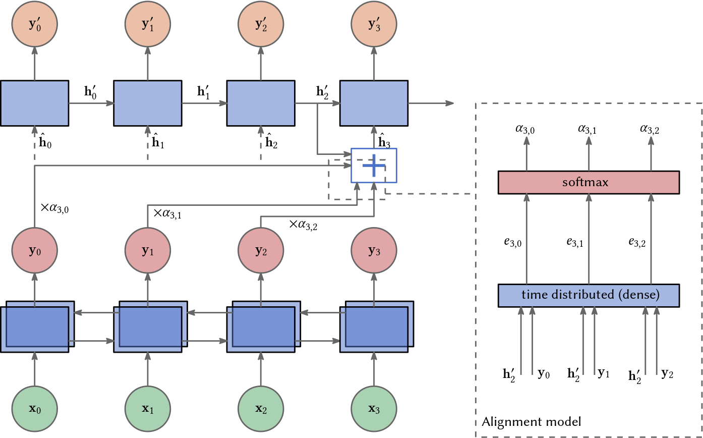
What is the idea behind the attention mechanism? Attention was introduced to bidirectional recurrent neural networks (RNNs) in 2014 (Bahdanau et al., 2014) for language translation, that is, for an encoder-decoder architecture. In this scenario we want to translate a sentence from e.g. English into e.g. German. The attention mechanism helps the decoder part of the RNN to focus on different parts of the encoder’s output (representations of the English words) differently. Therefore, it helps to preserve long term dependencies.
The encoder’s input is a sequence of tokens, let’s say words for simplicity, i.e. a sequence
\[\mathbf{x}_{0}, \ldots \mathbf{x}_{n-1}.\]For each word \(\mathbf{x}_{i}\) it computes some output \(\mathbf{y}_{i}\). The assumption is that the probability for \(\mathbf{x}_{i}\) depends on \(\mathbf{x}_{j}\). Since we have the whole sentence given, we can use a bidirectional RNN and look into the future. Thus, with respect to dependency, the probability for token \(i\) can depend on the probability for token \(j\) and vice versa.
The decoder’s input is the whole sequence computed by the encoder but as a weighted sum. The output is a sequence of German words, let’s say
\[\mathbf{y'}_{0}, \ldots \mathbf{y'}_{n-1}.\]This time however, the decoder RNN is unidirectional. It can not look into the future and computes each German word strictly from left to right. To compute the weights or attention scores of \(\mathbf{y'}_{i}\), an alignment model receives the hidden state \(\mathbf{h'}_{i-1}\) and the outputs of the encoder as input. First a simple dot product is computed:
\[e_{i,j} = \mathbf{h'}_{i}^\top \mathbf{y}_{j} \quad \text{ for } j = 0, \ldots, i-1.\]Later it was suggested to use an additional linear transformation on the output:
\[e_{i,j} = \mathbf{h'}_{i}^\top (\mathbf{W}\mathbf{y}_{j}) \quad \text{ for } j = 0, \ldots, i-1.\]where \(\mathbf{W}\) is learned. All these scores are normalized by the softmax function giving us \(n\) weights:
\[\alpha_{i,j} = \frac{\exp\left( e_{i,j} \right)}{\sum\limits_{k=0}^{n-1} \exp\left( e_{i, k}\right)}.\]Then the decoder’s ‘real’ input is computed by a weighted sum of the encoder’s output:
\[\hat{\mathbf{h}}_i = \sum_j \alpha_{i,j} \mathbf{y}_j.\]The weights determine how “strong” the information of the decoder’s input will be utilized, i.e., how much attention is spent on each previous output of the model.
This results in a quadratic complexity of \(\mathcal{O}(n^2)\) because for each of the \(n\) tokens, we want to decode, we have \(n\) weights.
The Transformer Architecture
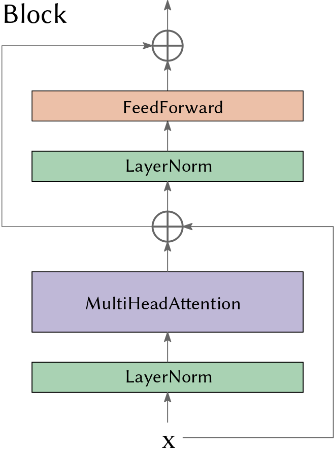
The original transformer was introduced for the task of machine translation thus it was an encoder-decoder architecture. In Fig. 2 you see a slightly modified version where the addition (residual connections) and the layer norm are in front of the attention layer.
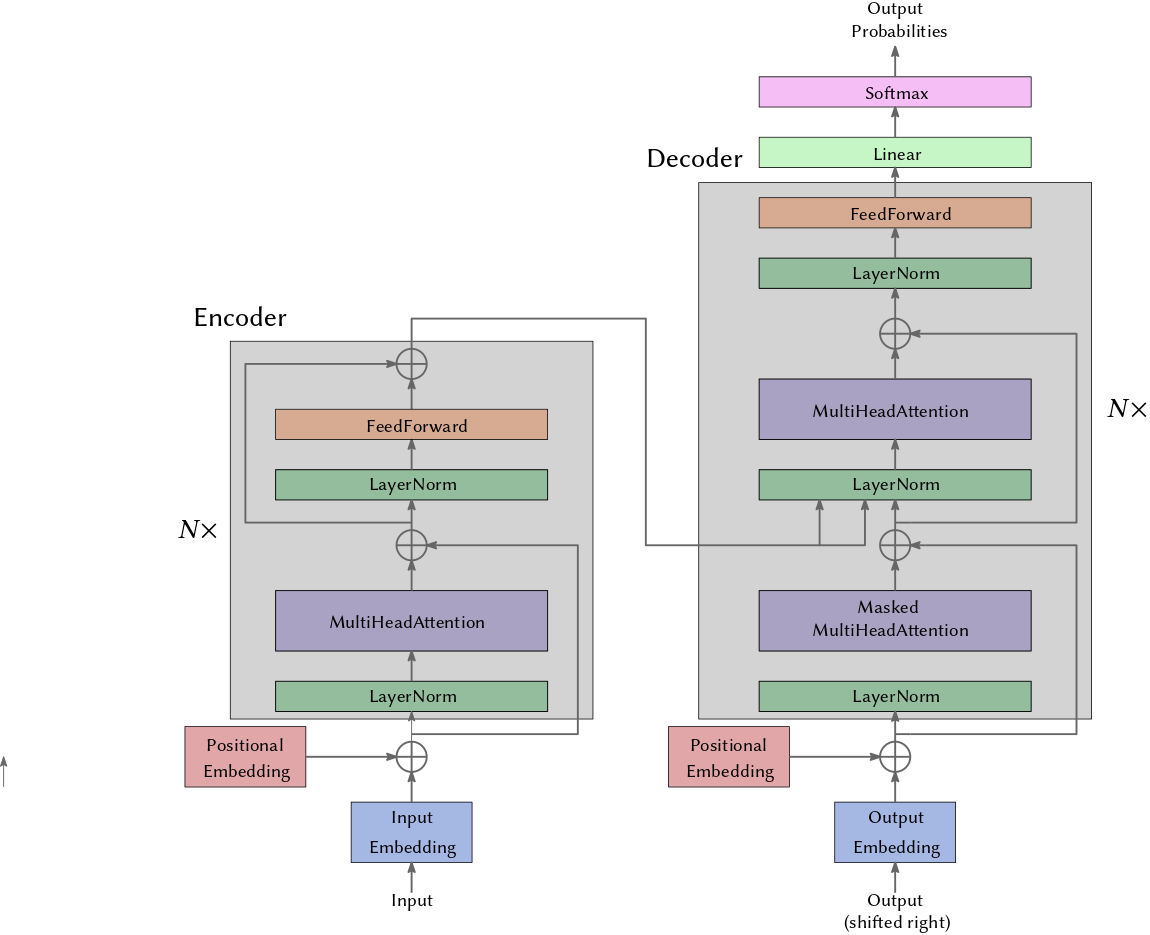
Let’s consider a scenario in which we have an English sentence that we want to translate into French. In this process, the encoder plays a crucial role by transforming the English sentence into a highly compressed and information-rich representation.
Subsequently, the decoder comes into play, generating the French translation word by word. It relies on the previously computed French words to predict and produce the next one. It’s important to note that the input provided to the decoder is a partial translation, essentially a shifted version of what it is currently working on. This is because the decoder should lack the ability to see into the future; it only has access to the portion of the translation it has computed up to that point—otherwise it would cheat while training which would hurt the learning process.
To address this limitation, the decoder employs a masked version of the multi-head attention layer. This mechanism ensures that the decoder focuses on the relevant information without peeking ahead.
Furthermore, the utilization of residual connections and layer normalization over the feature dimension within a single sample serves as a valuable tool to combat the issue of vanishing gradients in deep neural networks, ensuring the efficient training and optimization of the translation model.
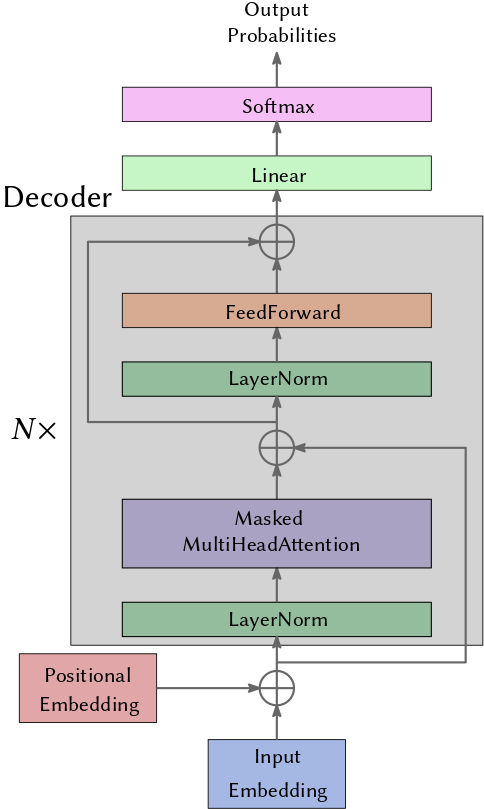
In our case we do not actually want to translate a sentence but we want to generate musical notes from a sequence of given notes. Therefore, we have no encoded information and there is no encoding involved. We only need the decoder part. Furthermore, I only use one (masked) multi-head attention layer in each block.
Ok, but how does this really work? What is going on here? Well, the key to understand transformers is to understand the self-attention mechanism which I try to explain below.
Self-Attention
The idea of the transformer is to just rely on (self-)attention thus remove recurrency. This means that the model “sees” \(n\) tokens to generate the \((n+1)^\text{th}\) token. Simple RNNs for predicting the next tokens only see the previous token and the hidden state which represents all the tokens before. But, as I discussed in previous articles, the information of the hidden state gets washed away over time and without attention there seems to be little control over the importance of certain tokens of the sequence.
The fundamental operation of the transformer, i.e. the attention mechanism, is implemented in its Head.
Let \(\mathbf{x}_0, \ldots, \mathbf{x}_{n-1} \in \mathbb{R}^{D \times 1}\) be the \(n\) tokens of a sequence.
A standard neural network layer \(f(\cdot)\), takes a \(D \times 1\) input and applies a linear transformation followed by an activation function like a \(\text{ReLU}\):
where \(\mathbf{b}\) contains the biases, and \(\mathbf{W}\) contains the weights.
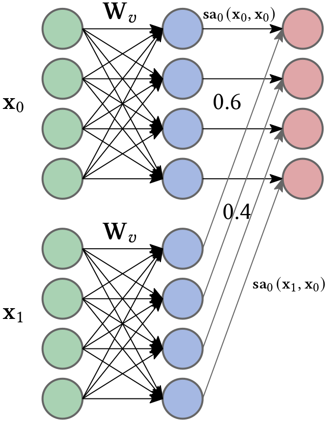
A self-attention \(\mathbf{sa}(\cdot)\) block takes all the \(n\) inputs, each of dimension \(D \times 1\), and returns \(n\) output vectors of the same size. Note that in our case each input represents a musical note or event. First, a set of values is computed for each input:
\[\mathbf{v}_i = \mathbf{b}_v + \mathbf{W}_v \mathbf{x}_i, \quad \text{ (value)}\]where \(\mathbf{b}_v \in \mathbb{R}^D \text{ and } \mathbf{W}_v \in \mathbb{R}^{D \times D}\) represent biases and weights, respectively (for all inputs). The \(j^\text{th}\) output \(\mathbf{sa}_j(\mathbf{x}_0, \ldots, \mathbf{x}_{n-1})\) is a weighted sum of all the values \(\mathbf{v}_i, i = 0, \ldots n-1\) where each weight depends on \(\mathbf{x}_j\):
\[\mathbf{sa}_j(\mathbf{x}_0, \ldots, \mathbf{x}_{n-1}) = \sum_{i=0}^{n-1} \alpha(\mathbf{x}_i, \mathbf{x}_j) \mathbf{v}_i.\]The scalar weight \(\alpha(\mathbf{x}_i, \mathbf{x}_j)\) is the attention that the \(j^\text{th}\) note pays to the note \(\mathbf{x}_i\). The \(n\) weights \(\alpha(\cdot, \mathbf{x}_j)\) are non-negative and sum to one. Hence, self-attention can be thought of as routing the values in different proportions to create each output.
To compute the attention, we apply two more linear transformations to the inputs:
\[\begin{aligned} \mathbf{q}_j &= \mathbf{b}_q + \mathbf{W}_q \mathbf{x}_j \quad \text{ (query)}\\ \mathbf{k}_i &= \mathbf{b}_k + \mathbf{W}_k \mathbf{x}_i \quad \text{ (key).} \end{aligned}\]The dot product of two vectors \(\mathbf{q}_j\), \(\mathbf{k}_i\) is a measurement of their similarity. The matrices \(\mathbf{W}_q, \mathbf{W}_k\) and the respective bias are learned such that similarity of \(\mathbf{q}_j\), \(\mathbf{k}_i\) can be interpreted as how “important” \(\mathbf{x}_i\) is for \(\mathbf{x}_j\). Thus, the “magic” happens via a very simple linear transformation and one might ask if this operation is powerful enough to relate all words/tokens in a desirable way. The answer is most certainly “no” thus one adds feed forward layers which introduce non-linearity in between multiple attention layers.
In the special case where both vectors are unit vectors, the dot product is the cosine of the angle between the two. In general, this relationship is expressed by the following equation:
\[\mathbf{q}_j \circ \mathbf{k}_i = \mathbf{q}_j^\top \mathbf{k}_i = \Vert \mathbf{q}_j \Vert \cdot \Vert \mathbf{k}_i \Vert \cos(\beta),\]where \(\beta\) is the angle between the two vectors. Computing the dot product between queries and keys gives us the similarities we desire. To normalize, we then pass the result through a softmax function:
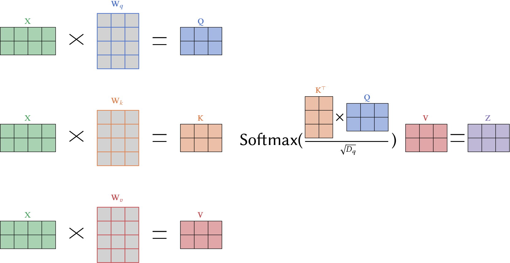
\[\alpha(\mathbf{x}_i, \mathbf{x}_j) = \frac{\exp(\mathbf{q}_j^\top \mathbf{k}_i / \sqrt{D_q})}{\sum\limits_{r=0}^{n-1} \exp(\mathbf{q}_j^\top \mathbf{k}_r / \sqrt{D_q})},\]where \(D_q\) is the dimension of the queries and keys (i.e., the number of rows in \(\mathbf{W}_q\) and \(\mathbf{W}_k\), which must be the same). You can think of the key as what is offered and the query as what is searched for. If \(\mathbf{X}\), \(\mathbf{K}\), \(\mathbf{Q}\), and \(\mathbf{V}\) contain all the inputs, keys, queries and values then we can compute the self-attention by
\[\mathbf{Sa}(\mathbf{X}) = \mathbf{V} \cdot \text{Softmax}\left( \frac{\mathbf{K}^\top \mathbf{Q}}{\sqrt{D_q} }\right).\]The overall computation is illustrated in Figure 5.
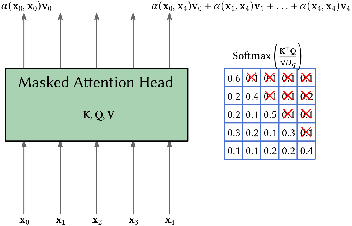
Masking Attention Head
Since our transformer should not look into the future, because when we use it in the prediction mode it also can not look ahead of the token it predicts, we have to mask entries in
\[\text{Softmax}\left(\frac{\mathbf{K}^\top \mathbf{Q}}{\sqrt{D_q}}\right).\]If you look into the code, I did this by setting the respective values in \(\mathbf{K}^\top \mathbf{Q}\) to negative infinity before computing the softmax.
class Head(nn.Module):
    """ one head of self-attention """

    def __init__(self, n_embd, head_size, sequence_len, dropout):
        super().__init__()
        self.key = nn.Linear(n_embd, head_size, bias=False)   # key embedding
        self.query = nn.Linear(n_embd, head_size, bias=False) # query embedding
        self.value = nn.Linear(n_embd, head_size, bias=False) # value embedding
        self.register_buffer('tril', torch.tril(torch.ones(sequence_len, sequence_len)))
        self.dropout = nn.Dropout(dropout) # to avoid overfitting

    def forward(self, x):
        B,T,C = x.shape
        k = self.key(x) # B, T, head_size, compute all keys
        q = self.query(x) # B, T, head_size, compute all queries
        _, _, head_size = q.shape

         # B, T, head_size @ B, head_size,
        wei = q @ k.transpose(-2, -1) * (head_size ** (-0.5)) # T => B, T, T

        # because we can not look into the future
        wei = wei.masked_fill(self.tril[:T, :T]==0, float('-inf'))
        wei = F.softmax(wei, dim=-1)
        wei = self.dropout(wei)

        v = self.value(x) # B, T, head_size
        out = wei @ v # T, T @ B, T, head_size => B, T, head_size
        return out
...
The multi-head attention layer consists of multiple heads. Note that apart from masked self-attention, the head also applies a dropout which helps with regularization.
Stacked Multi-Head Attention
Instead of using only one Head it is usually a good idea to use multiple ones.
To do this we transform the input into a head_size-dimensional space.
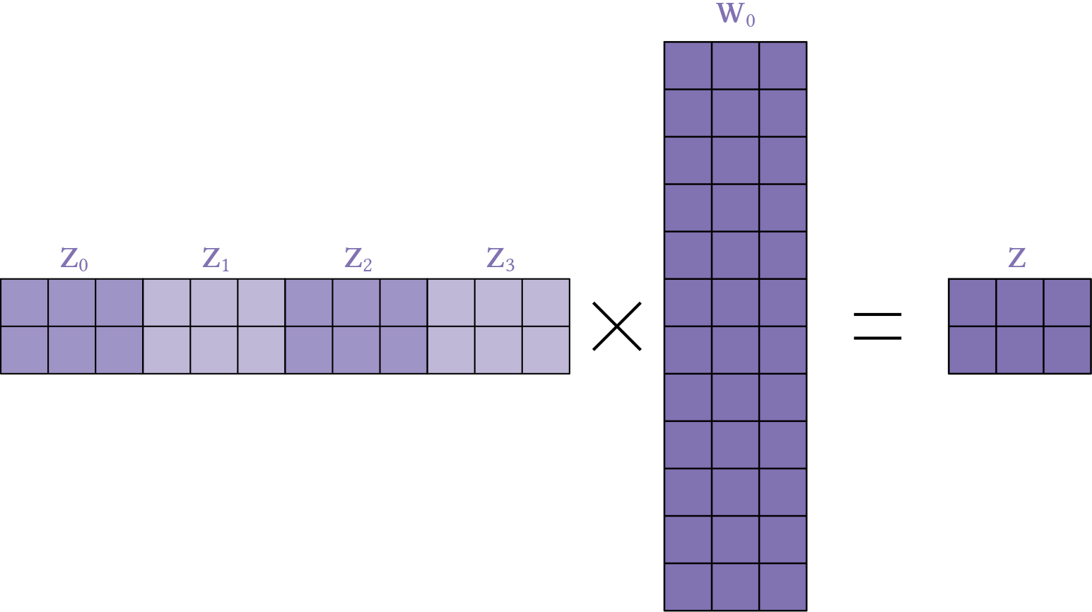
Suppose we use 4 heads then head_size * 4 should be equal to the rows of \(\mathbf{W}_0\) (compare Fig. 7) of the multi-head attention layer.
Since I add the input to the output of MultiHeadAttention (via residual connections), the columns of \(\mathbf{W}_0\) should be equal to the dimension of the input of the MultiHeadAttention.
In my case this is n_embd, i.e. the dimension of our embedded tokens.
\(\mathbf{W}_0\) transforms the concatenated results of the heads back to the dimension equal to n_embd.
This is needed to stack Blocks (each consisting of a MultiHeadAttention) on top of each other.
The output of Block \(i\) has to fit into block \(i+1\).
class MultiHeadAttention(nn.Module):
    def __init__(self, n_embd, n_heads, head_size, sequence_len, dropout):
        super().__init__()
        self.heads = nn.ModuleList(
            [Head(n_embd, head_size, sequence_len, dropout) for _ in range(n_heads)]
        )

        # W_0
        self.W0 = nn.Linear(head_size * n_heads, n_embd)

        self.dropout = nn.Dropout(dropout)

    def forward(self, x):
        # concatenation of the results of each head
        out = torch.cat([head(x) for head in self.heads], dim=-1)

        # Figure 7
        out = self.W0(out)
        out = self.dropout(out)
        return out
...
The hope is that each Head concentrates on different parts of the structure we want to learn.
Transformer Block
A Block consists of a MultiHeadAttention-layer and a relatively simple FFN-layer followed by two LayerNorm which applies layer normalization over the feature dimension within a single sample.
This helps the gradients to stay in a “good” range.
class Block(nn.Module):

    def __init__(self, n_embd, n_heads, sequence_len, dropout):
        super().__init__()
        # head_size could be defined differently
        head_size = n_embd // n_heads
        self.sa = MultiHeadAttention(n_embd, n_heads, head_size, sequence_len, dropout)
        self.ffwd = FeedForward(n_embd, dropout)
        self.ln1 = nn.LayerNorm(n_embd)
        self.ln2 = nn.LayerNorm(n_embd)

    def forward(self, x):
        x = x + self.sa(self.ln1(x)) # residual connection
        x = x + self.ffwd(self.ln2(x)) # residual connection
        return x

class FeedForward(nn.Module):

    def __init__(self, n_embd, dropout):
        super().__init__()
        self.net = nn.Sequential(
            nn.Linear(n_embd, 4 * n_embd),
            nn.ReLU(),
            nn.Linear(4 * n_embd, n_embd),
            nn.Dropout(dropout),
        )

    def forward(self, x):
        return self.net(x)
...
Positional Encoding
The Transformer has no more hidden state. Therefore, instead of processing token by token trying to memorize important information via the hidden state, it processes all \(n\) tokens in parallel, which is good for parallel computation but increases the time and space complexity from \(\mathcal{O}(n)\) (LSTM) to \(\mathcal{O}(n^2)\).
Furthermore, we have to encode the position of the tokens into \(\mathbf{x}\) because we lost the implicit order of computation. In the original paper (Vaswani et al., 2017) the authors utilized an embedding that involved sine and cosine functions. Their embedding is a very clever use of periodic functions but I will not go into details here. Instead of using a fixed embedding, I let the transformer learn the positional embedding.
Therefore, I transform the input idx into two vectors positional embedding and token embedding, which are added together.
Note that our input idx is an array of numbers each representing the id of the token.
Each number will be transformed into a specific vector (i.e. its embedding).
The embedding will be learned.
class TransformerDecoder(nn.Module):

    def __init__(self, vocab_size, sequence_len, n_embd, n_heads, n_blocks, dropout):
        super().__init__()

        # vocab_size is the size of our alphabet
        self.token_embedding_table = nn.Embedding(vocab_size, n_embd)

        # sequence_len is equal to n
        self.position_embedding_table = nn.Embedding(sequence_len, n_embd)

        self.blocks = nn.Sequential(
            *[Block(n_embd, n_heads, sequence_len, dropout) for _ in range(n_blocks)]
        )
        self.lm_head = nn.Linear(n_embd, vocab_size)

    def forward(self, idx):
        B, T = idx.shape

        # token embedding. B, T, n_embd
        token_emb = self.token_embedding_table(idx)

        # positional embedding. T, n_embd
        pos_emb = self.position_embedding_table(torch.arange(T, device=device))

        x = token_emb + pos_emb # B, T, n_embd + T, n_embd => B, T, n_embd
        x = self.blocks(x) # B, T, head_size
        logits = self.lm_head(x) # B, T, vocab_size
        return logits

...
By increasing the dimension of the embedding, the sequence length, the number of heads within a block and the number of blocks we can drastically increase the size and power of our decoder-only transformer. However, this will rapidly increase the memory requirements and training time.
Furthermore, it is very important to understand that what really matters is a high-quality training dataset! Of course, your model architecture matters too, but your model can not learn what is not there. Additionally, the musical representation you feed into the transformer matters as well. In our case this representation, using basically piano rolls, is very simple. It does not contain any high level information such as the end of a bar, section, phrase or musical theme. We just hope that the transformer will eventually learn all these concepts. It is an active research question what impact a good musical representation has on the result the trained transformer generates.
Relative Positional Self-Attention
So far our positional encoding was just a sequence of natural numbers \(0, 1, \ldots, n-1\) and we used an embedding which was added to the input, that is, the embedding of \(i\) was added to the embedding of \(\mathbf{x}_i\) of the input sequence. However, this encoding might not be optimal in the context of music where tones, phrases, musical ideas and themes repeat frequently. A relative position representation to allow attention to be informed by how far two positions are apart in a sequence might be much more effective.
So, instead of learning the index of a token within a sequence we want the model to learn relative distances between tokens. In other words, instead of learning the attention spent by token with index \(j\) on \(i\), that is, \(\alpha(\mathbf{x}_i, \mathbf{x}_j)\) we want to compute an attention score based on the (directed) distance \(i-j\). This concept was introduced by (Shaw et al., 2018).
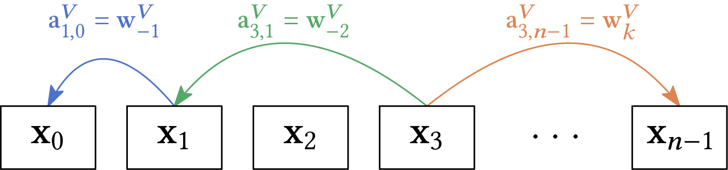
Note that if there are \(\mathcal{O}(n)\) absolute positions \(0, 1, \ldots, n-1\) then there are \(\mathcal{O}(n)\) relative positions \(-(n-1), \ldots, -1, 0, 1,\ldots, n-1\). The authors also introduce a maximal distance \(k\) such that they only learn weights
\[\mathbf{w}^{V}_{\text{clip}(i-j,k)} \text{ with } \text{clip}(x,k) = \max(-k, \min(k,x))\]Therefore, they learn relative position representations for the keys \(\mathbf{w}^K_{-k}, \ldots, \mathbf{w}^K_{k}\) and for the values \(\mathbf{w}^V_{-k}, \ldots, \mathbf{w}^V_{k}\). They introduce the relative position between \(\mathbf{x}_i\) and \(\mathbf{x}_j\) to be
\[\mathbf{a}_{ij} = \mathbf{w}_{\text{clip}(i-j,k)}\]Thus there are \(\mathcal{O}(n^2)\) different such vectors but many share the same value. Of course, they drop the absolute positional encoding. And they adapt the self-attention computation from
\[\mathbf{sa}_j(\mathbf{x}_0, \ldots, \mathbf{x}_{n-1}) = \sum_{i=0}^{n-1} \alpha(\mathbf{x}_i, \mathbf{x}_j) \mathbf{v}_i.\]to
\[\mathbf{sa}_j(\mathbf{x}_0, \ldots, \mathbf{x}_{n-1}) = \sum_{i=0}^{n-1} \alpha(\mathbf{x}_i, \mathbf{x}_j) (\mathbf{v}_i + \mathbf{a}^V_{ij}).\]and the computation of the similarity between query and key from
\[\frac{(\mathbf{W}_q \mathbf{x}_j)^\top (\mathbf{W}_k \mathbf{x}_i)}{\sqrt{D_q}}\]to
\[\frac{(\mathbf{W}_q \mathbf{x}_j)^\top (\mathbf{W}_k \mathbf{x}_i + \mathbf{a}^K_{ij})}{\sqrt{D_q}}.\]Computation-wise the first manipulation can be easily achieved by adding a matrix \(\mathbf{A}\) to \(\mathbf{V}\). However, the second manipulation destroys parallelism, i.e. the possibility to compute everything by matrix-matrix multiplications. This can be mitigated by splitting the computation into two parts:
\[\frac{(\mathbf{W}_q \mathbf{x}_j)^\top (\mathbf{W}_k \mathbf{x}_i + \mathbf{a}^K_{ij})}{\sqrt{D_q}} = \frac{(\mathbf{W}_q \mathbf{x}_j)^\top (\mathbf{W}_k \mathbf{x}_i) + (\mathbf{W}_q \mathbf{x}_j)^\top \mathbf{a}^K_{ij}}{\sqrt{D_q}}\]Assuming that \(\mathbf{S}\) contains all the relative attention scores, that is,
\[\mathbf{S}_{ij} = (\mathbf{W}_q \mathbf{x}_j)^\top \mathbf{a}^K_{ij},\]then we can go back to the matrix form which gives us
\[\mathbf{Sa}(\mathbf{X}) = (\mathbf{V} + \mathbf{A}^V) \cdot \text{Softmax}\left( \frac{\mathbf{K}^\top \mathbf{Q} + \mathbf{S}}{\sqrt{D_q} }\right).\]To compute \(\mathbf{S}\) (Shaw et al., 2018) instantiate an intermediate tensor \(\mathbf{R} \in \mathbf{R}^{k \times k \times D_q},\) containing the embeddings that correspond to the relative distance between all keys and queries. \(\mathbf{Q}\) is then reshaped to an \((k, 1, D_q)\) tensor, and \(\mathbf{S} = \mathbf{Q} \mathbf{R}^\top.\) This incurs a total space complexity of \(\mathcal{O}(k^2 D_q)\).
The Music Transformer
The Music Transformer (Huang et al., 2018) was one of the first transformer utilized to generate symbolic music. Even if it was introduced five years ago (which is like a century in the AI-world) it is worth studying it. In the paper you find two different datasets
and they used an impressive sequence length of 2048-tokens! They used GPUs for the training. With such a large number of token, one question arises: How did they manage to put 2000-tokens and all the respective matrices in the GPUs’ memory?
The authors correctly identify the space complexity of \(\mathcal{O}(k^2 D_q)\) to be problematic for GPU computation and they reduce the complexity to \(\mathcal{O}(k D_q)\) by exchanging space for re-computation. This is possible due to the structure of the tensor \(\mathbf{R}\) which contains many equal values.
To handle very long sequences, the authors use local attention (Liu et al., 2018) by chunking the input sequence into non-overlapping blocks. Each block then attends to itself and the one before.
Attention-Free Transformer
Basically, the attention mechanism, regardless of the specifics, solves a routing problem, that is, which information is transported to the next layer of the neural network. Thus, it has a quadratic time and space complexity of \(\mathcal{O}(n^2)\) where \(n\) is our sequence length. Therefore, if you have limited resources, it is hard to scale it to larger sequences. As with the local attention and other techniques, like the Linformer (Wang et al., 2020), Longformer (Beltagy et al., 2020), Reformer (Kitaev et al., 2020), and Synthesizer (Tay et al., 2021), and Performer (Choromanski et al., 2022) there are ways to improve this but in principle the complexity will bite us eventually.
Now we enter in an era in deep learning where we question if we actually need the attention layers in the transformer!
This was proposed in 2022.
Instead of computing attention, FNet (Lee-Thorp et al., 2022) just mixes tokens according to the discrete Fourier transformation (DFT).
First, a 1D transformation is computed with respect to the embedding and then another with respect to time.
Amazingly even though there is no parameter to learn within the Fourier-layer (which replaces the Head) this strategy seems to work almost as good as the far more computationally expensive task of learning all the required attention scores.
The Fourier transform decomposes a function (in our case a discrete signal) into its constituent frequencies. Given a sequence \(x_0, \ldots, x_{N-1}\), the discrete Fourier transform (DFT) is defined by
\[X_k = \sum\limits_{n=0}^{N-1} x_n \exp\left( - \frac{2\pi i}{N} nk \right), \quad 0 \leq k \leq N-1.\]\(X_k\) encodes the phase and amplitude of frequency \(k\) within the signal.
FNet consists of a Fourier mixing sublayer followed by a feed-forward sublayer. Essentially, the self-attention sublayer of each transformer decoder layer is replaced with a Fourier sublayer which applies a 2D DFT to its
\[(\text{sequence length} \times \text{hidden dimension})\]embedding input. This can be achieved using two 1D DFTs—one 1D DFT along the sequence dimension, \(\mathcal{F}_\text{seq}\), and one 1D DFT along the hidden dimension, \(\mathcal{F}_\text{h}\):
\[y = \text{Real}\left( \mathcal{F}_\text{seq} \left( \mathcal{F}_\text{h}(\mathbf{x}) \right) \right)\]The authors only consider the real part of the DFT.
Now, as emphasized by the title of their paper, the Fourier transform is probably not the important part. It is just a special case of how you can mix tokens. Important is the mixing itself which allows information to flow from one token to all the other tokens and the Fourier transform happens to be a nice way of mixing. The paper indicates that it might not be so important to let the model learn how exactly information flows around. It might be just enough if information flows at all (to all tokens). In other words, the exact routing might be less important than we thought.
Now, the results of the paper are not better than using a traditional transformer. But one trades accuracy for resources thus longer sequence length and a faster computation.
To the best of my knowledge, I have not seen this tried out for symbolic music generation. But when I have time, I’ll play around with it. Furthermore, one might think about a special mixing which is effective for our specific task.
References
- Vaswani, A., Shazeer, N., Parmar, N., Uszkoreit, J., Jones, L., Gomez, A. N., Kaiser, L., & Polosukhin, I. (2017). attention is all you need. CoRR, abs/1706.03762. http://arxiv.org/abs/1706.03762
- Hochreiter, S., & Schmidhuber, J. (1997). Long short-term memory. Neural Computation, 9(8), 1735–1780. https://doi.org/10.1162/neco.1997.9.8.1735
- Chung, J., Gulcehre, C., Cho, K. H., & Bengio, Y. (2014). Empirical evaluation of gated recurrent neural networks on sequence modeling.
- Bahdanau, D., Cho, K., & Bengio, Y. (2014). Neural machine translation by jointly learning to align and translate. CoRR, abs/1409.0473.
- Brown, T. B., Mann, B., Ryder, N., Subbiah, M., Kaplan, J., Dhariwal, P., Neelakantan, A., Shyam, P., Sastry, G., Askell, A., Agarwal, S., Herbert-Voss, A., Krueger, G., Henighan, T., Child, R., Ramesh, A., Ziegler, D. M., Wu, J., Winter, C., … Amodei, D. (2020). Language models are few-shot learners.
- OpenAI. (2023). GPT-4 rechnical report.
- Bubeck, S., Chandrasekaran, V., Eldan, R., Gehrke, J., Horvitz, E., Kamar, E., Lee, P., Lee, Y. T., Li, Y., Lundberg, S., Nori, H., Palangi, H., Ribeiro, M. T., & Zhang, Y. (2023). Sparks of artificial general intelligence: Early experiments with GPT-4.
- Touvron, H., Lavril, T., Izacard, G., Martinet, X., Lachaux, M.-A., Lacroix, T., Rozière, B., Goyal, N., Hambro, E., Azhar, F., Rodriguez, A., Joulin, A., Grave, E., & Lample, G. (2023). LLaMA: Open and efficient foundation language models.
- Touvron, H., Martin, L., Stone, K., Albert, P., Almahairi, A., Babaei, Y., Bashlykov, N., Batra, S., Bhargava, P., Bhosale, S., Bikel, D., Blecher, L., Ferrer, C. C., Chen, M., Cucurull, G., Esiobu, D., Fernandes, J., Fu, J., Fu, W., … Scialom, T. (2023). LlaMA 2: Open foundation and fine-tuned chat models.
- Devlin, J., Chang, M.-W., Lee, K., & Toutanova, K. (2019). BERT: Pre-training of deep bidirectional transformers for language understanding.
- Chen, M., Tworek, J., Jun, H., Yuan, Q., de Oliveira Pinto, H. P., Kaplan, J., Edwards, H., Burda, Y., Joseph, N., Brockman, G., Ray, A., Puri, R., Krueger, G., Petrov, M., Khlaaf, H., Sastry, G., Mishkin, P., Chan, B., Gray, S., … Zaremba, W. (2021). Evaluating large language models trained on code.
- Huang, C.-Z. A., Vaswani, A., Uszkoreit, J., Shazeer, N., Hawthorne, C., Dai, A. M., Hoffman, M. D., & Eck, D. (2018). Music Transformer: Generating music with long-term structure. ArXiv Preprint ArXiv:1809.04281.
- Huang, Y.-S., & Yang, Y.-H. (2020). Pop Music Transformer: Beat-based modeling and generation of expressive pop piano compositions.
- Ens, J., & Pasquier, P. (2020). MMM: Exploring conditional multi-track music generation with the transformer.
- Hadjeres, G., & Crestel, L. (2021). The piano inpainting application.
- Shih, Y.-J., Wu, S.-L., Zalkow, F., Müller, M., & Yang, Y.-H. (2022). Theme Transformer: Symbolic music generation with theme-conditioned transformer.
- Copet, J., Kreuk, F., Gat, I., Remez, T., Kant, D., Synnaeve, G., Adi, Y., & Défossez, A. (2023). Simple and controllable music generation.
- Shaw, P., Uszkoreit, J., & Vaswani, A. (2018). Self-attention with relative position representations. CoRR, abs/1803.02155. http://arxiv.org/abs/1803.02155
- Liu, P. J., Saleh, M., Pot, E., Goodrich, B., Sepassi, R., Kaiser, L., & Shazeer, N. (2018). Generating Wikipedia by summarizing long sequences. International Conference on Learning Representations. https://openreview.net/forum?id=Hyg0vbWC-
- Wang, S., Li, B. Z., Khabsa, M., Fang, H., & Ma, H. (2020). Linformer: Self-Attention with linear complexity.
- Beltagy, I., Peters, M. E., & Cohan, A. (2020). Longformer: The long-document transformer.
- Kitaev, N., Kaiser, Ł., & Levskaya, A. (2020). Reformer: The Efficient Transformer.
- Tay, Y., Bahri, D., Metzler, D., Juan, D.-C., Zhao, Z., & Zheng, C. (2021). Synthesizer: Rethinking self-attention in transformer models.
- Choromanski, K., Likhosherstov, V., Dohan, D., Song, X., Gane, A., Sarlos, T., Hawkins, P., Davis, J., Mohiuddin, A., Kaiser, L., Belanger, D., Colwell, L., & Weller, A. (2022). Rethinking Attention with Performers. https://arxiv.org/abs/2009.14794
- Lee-Thorp, J., Ainslie, J., Eckstein, I., & Ontanon, S. (2022). FNet: Mixing tokens with Fourier transforms.