Musical Interrogation III - LSTM
This article is Part 3 in a 4-Part Series.
- Part 1 - Musical Interrogation I - Intro
- Part 2 - Musical Interrogation II - MC and FFN
- Part 3 - Musical Interrogation III - LSTM
- Part 4 - Musical Interrogation IV - Transformer
This article is the continuation of a series. It is recommended that you read part I and II first. This time we use a recurrent neural network (RNN), more precisely an LSTM, which I explained a little bit in the introduction. An LSTM is a RNN that counteracts the problem of exploding and vanishing gradients.
This article gives some explanation to the code in the following notebook, which can be executed on Google Colab.
Because our model is now able to learn long-time relations, we can use the GridEncoder, i.e., a piano roll data representation, which is exactly what we do.
Recurrent Neural Networks
Prior to the advent of transformers, many cutting-edge natural language processing (NLP) applications relied on recurrent neural networks (RNNs). These networks are particularly adept at processing sequences of data, such as words in NLP tasks or notes and musical events in audio processing.
An RNN processes a sequence
\[\mathbf{x}_0, \ldots, \mathbf{x}_{n-1}\]of inputs one at a time. With each new input, the network not only considers this current input but also incorporates a hidden state—a representation of previous inputs—thanks to its recurrent connections. This hidden state \(\mathbf{h}_t\) is updated at each step, ensuring that the network retains a memory of what it has processed so far.
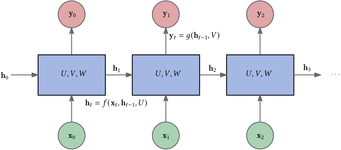
The unique feature of RNNs is their ability to maintain an internal state that captures information about the sequence they have processed to that point. As a result, the final output of the RNN is informed by the entire input sequence.
Furthermore, RNNs have been employed in sequence generation or decoding tasks. In such applications, the tokens generated by the RNN are fed back into it as inputs. This feedback loop allows the RNN to generate sequences where each new token is influenced by the previously generated tokens, making it suitable for tasks like text generation, music composition, and more.
Long Short-Term Memory Networks
Long short-term memory networks (LSTMs) are a type of RNN that were designed to overcome some of the limitations of vanilla RNNs, particularly in handling long-term dependencies in sequence data.
Vanilla RNNs struggle with learning long-term dependencies due to the vanishing gradient problem. As the length of the input sequence increases, the gradients used in the training process can become extremely small, making it difficult for the RNN to learn and retain information from earlier inputs. LSTMs address this issue with their unique architecture, which includes memory cells which uses different gates.
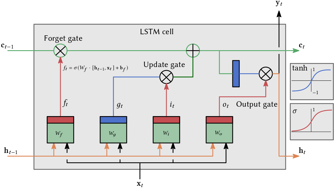
A memory cell can maintain information in memory for long periods of time. The key components of an such a cell are its gates: the input gate, output gate, and forget gate. These gates regulate the flow of information into and out of the cell, and they decide what to retain or discard from the cell state.
- Update Gate: Determines how much of the new information to add to the cell state.
- Forget Gate: Decides what information is no longer needed and removes it from the cell state, helping to prevent the accumulation of irrelevant information.
- Output Gate: Controls the extent to which the value in the cell is used to compute the output activation of the block.
Due to their architecture, LSTMs can learn and remember over longer sequences than vanilla RNNs, making them more effective for tasks like language modeling, text generation, speech recognition, and more, where understanding context over a long sequence is crucial. The gating mechanism helps mitigate the vanishing gradient problem, allowing for more effective training over longer sequences. This is because the gates allow gradients to flow through the network without being multiplied repeatedly by small numbers (which is what causes the gradients to vanish in vanilla RNNs).
Data Preparation
Again we use the data from EsAC.
The specific dataset I utilized is Folksongs from the continent of Europe and for the purpose of this work, I will exclusively use the 1700 pieces found in the ./deutschl/erk directory.
We assume that 1/16 is the shortest note in our dataset.
The GridEncoder automatically filters out pieces that do not fulfill this condition.
time_step = 1/16
encoder = GridEncoder(time_step)
enc_songs, invalid_song_indices = encoder.encode_songs(scores)
print(f'there are {len(enc_songs)} valid songs and {len(invalid_song_indices)} songs')
Let us look at an example encoded of a piece:
55 _ _ _ 60 _ _ _ 60 _ _ _ 60 _ _ _ 60 _ _ _ 64 _ _ _ 64 _ _ _ r _ _ _ 62 _ 64 _ 65 ...
As we discussed in the last article, 55 _ _ _ stands for the midinote 55 played for 4 beats where one beat is 1/16 note.
Therefore, this is a 1/4 note.
Likewise, r _ _ _ is a 1/4 rest.
Next, the StringToIntEncoder converts our alphabet of tokens into positive integers.
string_to_int = StringToIntEncoder(enc_songs)
Next, we use ScoreDataset to arrange our training data.
It requires our encoded songs, the instance of StringToIntEncoder and a hyperparameter sequence_len that configures the length of token sequences our model will be trained on.
The longer the sequence, the longer the training will require because the deeper the recurrent neural network will be.
sequence_len = 64 # this is a hyperparameter!
dataset = ScoreDataset(
    enc_songs=enc_songs,
    stoi_encoder=string_to_int,
    sequence_len=sequence_len)
It is now possible to split our data into training, validation and test set.
train_set, val_set, test_set = torch.utils.data.random_split(dataset, [0.8, 0.1, 0.1])
Model Definition
First we define the rest of our hyperparameters:
vocab_size = len(string_to_int) # size of our alphabet
input_dim = vocab_size # can be different
hidden_dim = 128 # can be different
layer_dim = 1 # can be different
output_dim = vocab_size # should not be different
dropout = 0.2 # can be different

criterion = torch.nn.CrossEntropyLoss()

learning_rate = 0.001 # can be different
batch_size = 64 # can be different
n_epochs = 10 # can be different
eval_interval = 100 # can be different
Before explaining every detail, let us look at the model definition first. The following is the model description of our RNN/LSTM. To understand what’s going on, look at the forward method. This sends our data through the network.
The first two lines create the short-term \(\mathbf{h}_0\) and long-term memory \(\mathbf{c}_0\) and fill them with zeros.
Then an embedding takes place: x = self.embedding(x).
This is nothing more than what we did with our simple feedforward net in Part II - FNN: Each element of the input x is first one-hot encoded and then multiplied by a matrix.
The result: Each event is represented by the row of a matrix (with learnable parameters).
The matrix has vocab_size rows and input_dim columns.
Next, we send our transformed input through our LSTM out, (ht, ct) = self.lstm(x, (h0, c0)).
This basically computes \(\mathbf{h}_t, \mathbf{c}_t\) based on \(\mathbf{h}_{t-1}, \mathbf{c}_{t-1}\) as indicated in Fig. 2.
We get as many outputs as our sequence is long, i.e., sequence_len many.
But we are only interested in the last output, which we get by out[:, -1, :].
This is a vector with hidden_dim elements.
We don’t need ht and ct.
Then we send the last output through a dropout layer to counteract overfitting.
In the last step, we transform the hidden_dim-dimensional vector into an output_dim-dimensional vector, which is equal to vocab_size.
This vector is interpreted as a probability distribution.
class LSTMModel(torch.nn.Module):
    def __init__(self, input_dim, hidden_dim, layer_dim, output_dim, dropout=0.2):
        super(LSTMModel, self).__init__()

        self.hidden_dim = hidden_dim
        self.layer_dim = layer_dim

        self.embedding = torch.nn.Embedding(vocab_size, input_dim)
        self.lstm = torch.nn.LSTM(input_dim, hidden_dim, layer_dim, batch_first=True)
        self.dropout = torch.nn.Dropout(dropout)
        self.fc = torch.nn.Linear(hidden_dim, output_dim)

    def forward(self, x):
        h0 = torch.zeros(self.layer_dim, x.size(0), self.hidden_dim, device=device)
        c0 = torch.zeros(self.layer_dim, x.size(0), self.hidden_dim, device=device)

        # x = B, T, C
        x = self.embedding(x)

        out, (ht, ct) = self.lstm(x, (h0, c0))
        out = self.dropout(out[:, -1, :])
        out = self.fc(out)
        return out # B, C
Next, we initialize the model:
model = LSTMModel(input_dim, hidden_dim, layer_dim, output_dim, dropout)
model.to(device)  # use gpu if possible

optimizer = torch.optim.Adam(model.parameters(), lr=learning_rate)

for i in range(len(list(model.parameters()))):
    print(list(model.parameters())[i].shape)
We could play with different hyperparameters.
Increasing hidden_dim basically increases the complexity of the “memory” of the LSTM.
We surely want to increase n_epochs to increase number of times the LSTM “sees” all training data.
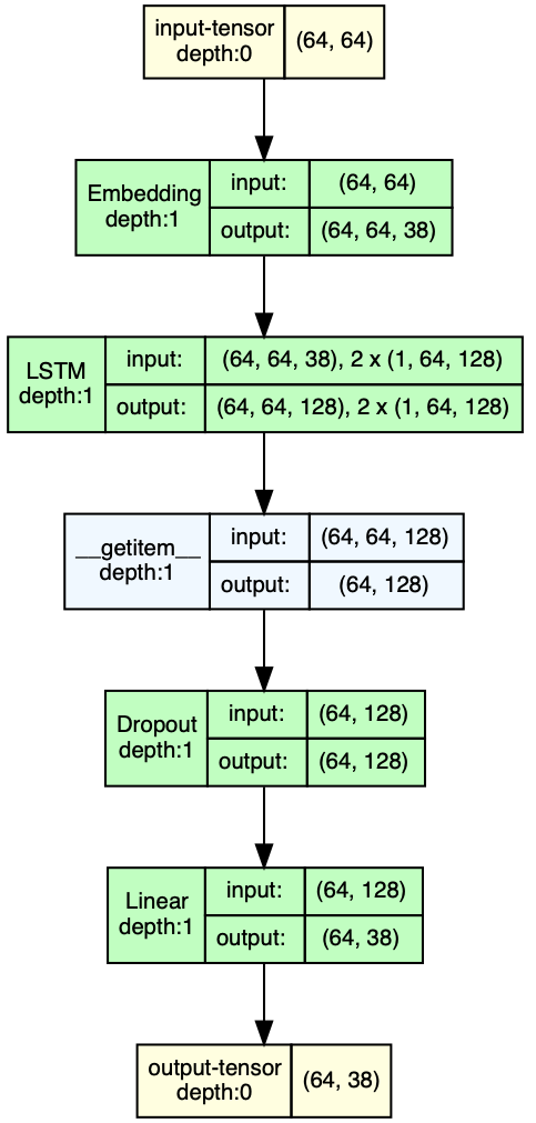
We can visualize the LSTM by utilizing the draw_graph function from the torchview package.
# (batch_size, sequence_len)
X_vis, y_vis = train_set[0:batch_size]
print(f'shape of X_vis: {X_vis.shape}')
print(f'shape of y_vis: {y_vis.shape}')
print(f'number of different symbols {vocab_size}')
X_vis, y_vis = X_vis.to(device), y_vis.to(device)
model_vis = LSTMModel(input_dim, hidden_dim, layer_dim, output_dim, dropout)
model_graph = draw_graph(model_vis, input_data=X_vis, device=device)
model_graph.visual_graph
Note that the softmax is part of our loss criterion i.e. the cross entropy loss torch.nn.CrossEntropyLoss() which is part of the backpropagation, i.e., the training process.
Melody Generation (Before Training)
Given a sequence of arbitrary length, the generate function is used to generate a new piece of music.
temperature determines how much the probability distribution learned by the model is considered.
temperatureequal to 1.0 means that sampling is done from the probability distribution.temperatureapproaching infinity means that sampling is done uniformly (more variation).temperatureapproaching 0 means that higher probabilities are emphasized (less variation).
We can set a maximum length for the piece and also provide the beginning of a piece.
def next_event_number(idx, temperature:float):
    with torch.no_grad():
        logits = model(idx)
        probs = F.softmax(logits / temperature, dim=1) # B, C
        idx_next = torch.multinomial(probs, num_samples=1)
        return idx_next

def generate(seq: list[str]=None, max_len:int=None, temperature:float=1.0):
    with torch.no_grad():
        generated_encoded_song = []
        if seq != None:
            idx = torch.tensor(
                [[string_to_int.encode(char) for char in seq]],
                device=device
            )
            generated_encoded_song = seq.copy()
        else:
            idx = torch.tensor([[string_to_int.encode(TERM_SYMBOL)]], device=device)

        while max_len == None or max_len > len(generated_encoded_song):
            idx_next = next_event_number(idx, temperature)
            char = string_to_int.decode(idx_next.item())
            if idx_next == string_to_int.encode(TERM_SYMBOL):
                break
            idx = torch.cat((idx, idx_next), dim=1) # B, T+1, C
            generated_encoded_song.append(char)

        return generated_encoded_song
Of course, the results are almost random because the parameters of our model are initialized randomly and we did not train it yet. The following code snippet generates 5 scores.
# number of songs we want to generate
n_scores = 5
temperature = 0.6
before_new_songs = []
for _ in range(n_scores):
    encoded_song = generate(max_len=13,temperature=temperature)
    print(f'generated {" ".join(encoded_song)} consisting of {len(encoded_song)} notes')
    before_new_songs.append(encoded_song)
Let’s listen to the first one:
Training
For training, we use something called a DataLoader.
This helps us to access our data more easily.
For example, we shuffle our data before training.
train_loader = DataLoader(train_set, batch_size=batch_size, shuffle=True)
val_loader = DataLoader(val_set, batch_size=batch_size, shuffle=True)
test_loader = DataLoader(test_set, batch_size=batch_size,shuffle=True)
The code for training seems a bit complicated because we use batches.
This is due to dealing with a large amount of data, and we don’t send all of it through the network at once (per training step), but only a part of it, namely batch_size many.
An epoch is defined by the fact that all training data have been sent through the network once.
In essence, nothing else happens but:
- Send Batch through the network (Forward pass)
- Calculate error/cost
- Propagate gradients of the cost function with respect to the model parameters backwards through the network (Backward pass)
- Update model parameters
def train_one_epoch(epoch_index, tb_writer, n_epochs):
    running_loss = 0.0
    last_loss = 0.0
    all_steps = n_epochs * len(train_loader)

    for i, data in enumerate(train_loader):
        local_X, local_y = data
        local_X, local_y = local_X.to(device), local_y.to(device)
        optimizer.zero_grad()
        outputs = model(local_X)

        loss = criterion(outputs, local_y)
        loss.backward()
        optimizer.step()

        running_loss += loss.item()
        if i % eval_interval == eval_interval-1:
            last_loss = running_loss / eval_interval

            steps = epoch_index * len(train_loader) + (i+1)

            ep_str = f'Epoch [{epoch_index+1}/{n_epochs}]'
            step_str = f'Step [{steps}/{all_steps}]'
            loss_str = f'Loss: {last_loss:.4f}'
            print(f'{ep_str}, {step_str}, {loss_str}')

            tb_x = epoch_index * len(train_loader) + i + 1
            tb_writer.add_scalar('Loss/train', last_loss, tb_x)
            running_loss = 0.

    return last_loss

# Initializing in a separate cell so we can easily add more epochs to the same run
def train(n_epochs,respect_val=False):
    timestamp = datetime.now().strftime('%Y%m%d_%H%M%S')
    writer = SummaryWriter('runs/fashion_trainer_{}'.format(timestamp))
    best_vloss = 1_000_000

    for epoch in range(n_epochs):
        model.train(True)
        avg_loss = train_one_epoch(epoch, writer, n_epochs)

        model.train(False)
        running_vloss = 0.0

        for i, vdata in enumerate(val_loader):

            local_X, local_y = vdata
            local_X, local_y = local_X.to(device), local_y.to(device)

            voutputs = model(local_X)
            vloss = criterion(voutputs, local_y)
            running_vloss += vloss

        avg_vloss = running_vloss / (i+1)

        ep_str = f'Epoch [{epoch+1}/{n_epochs}]'
        tloss_str = f'Train-Loss: {avg_loss:.4f}'
        vloss_str = f'Val-Loss: {avg_vloss:.4f}'
        print(f'{ep_str}, {tloss_str}, {vloss_str}')

        writer.add_scalars(
            'Training vs. Validation Loss',
            {'Training': avg_loss, 'Validation': avg_vloss},
            epoch
        )

        writer.flush()

        if not respect_val or (respect_val and avg_vloss < best_vloss):
            best_vloss = avg_vloss
            model_path = './models/_model_{}_{}'.format(timestamp, epoch)
            torch.save(model.state_dict(), model_path)
Calling train starts the training.
train(n_epochs)
The best model from the training can be found in the folder ./models and can be loaded as follows
model_path = './models/pretrained_1_128_best_val'

if device.type == 'cpu':
    model.load_state_dict(torch.load(model_path, map_location=torch.device('cpu')))
elif torch.backends.mps.is_available():
    model.load_state_dict(torch.load(model_path, map_location=torch.device('mps')))
else:
    model.load_state_dict(torch.load(model_path))
model.eval()
Melody Generation (After Training)
After training or after we load our pretrained model, we generate new pieces:
n_scores = 5
temperature = 0.6
after_new_songs = []
for _ in range(n_scores):
    encoded_song = generate(max_len=120,temperature=temperature)
    print(f'generated {" ".join(encoded_song)} consisting of {len(encoded_song)} notes')
    after_new_songs.append(encoded_song)

after_generated_scores = encoder.decode_songs(after_new_songs)
Audio(score_to_wav(after_generated_scores[0], 'a_g_song.wav'))
We start to hear repetition and some structure within the piece:
Real World Example
In the realm of musical innovation, a significant advancement occurred with the development of a sophisticated LSTM model designed to create expressive piano roll music. This model was introduced in a notable study by (Oore et al., 2018). The researchers devised a unique discrete-event based representation for piano rolls, encompassing a diverse range of 413 different events. The architecture of their model was meticulously structured, comprising three hidden LSTM layers, each equipped with 512 cells. This design choice facilitated the processing of a 413-dimensional one-hot vector as input, with the model subsequently generating a categorical distribution over the same dimensional space.
The training process of the model was finely tuned, employing a mini-batch size of 64 and a learning rate of 0.001, alongside the implementation of teacher forcing techniques. For those interested in experiencing the model’s capabilities firsthand, a collection of generated music pieces is available for listening at this link. However, it’s important to note a primary limitation of this model: its tendency to produce relatively brief musical compositions, typically ranging from 10 to 20 seconds in duration. The authors also emphasized the critical role of high-quality data in achieving optimal results with this model.
Following this development, the field witnessed the emergence of the Music Transformer, introduced by (Huang et al., 2018). This model also utilized a similar piano roll representation but marked a significant leap forward by employing the transformer architecture. This innovative approach enabled the Music Transformer to learn and reproduce longer sequences, demonstrating the capability to capture more extended musical dependencies. The transformer architecture and its implications in music generation will be further explored in the next installment of this series.
References
- Oore, S., Simon, I., Dieleman, S., Eck, D., & Simonyan, K. (2018). This time with feeling: Learning expressive musical performance.
- Huang, C.-Z. A., Vaswani, A., Uszkoreit, J., Shazeer, N., Hawthorne, C., Dai, A. M., Hoffman, M. D., & Eck, D. (2018). Music Transformer: Generating music with long-term structure. ArXiv Preprint ArXiv:1809.04281.