Musical Interrogation II - MC and FFN
This article is Part 2 in a 4-Part Series.
- Part 1 - Musical Interrogation I - Intro
- Part 2 - Musical Interrogation II - MC and FFN
- Part 3 - Musical Interrogation III - LSTM
- Part 4 - Musical Interrogation IV - Transformer
The code shown here can be found in the following GitHub repository. In the second installment of this series, I introduce an initial and arguably the most basic method to generate monophonic melodies. This consists of two approaches: (1) A first-order Markov chain (MC) and (2) a feedforward neural network (FNN)
It’s important to note that I will disregard all forms of dynamics within a notated score (or performance), such as loudness, softness, etc.
Despite these two approaches being significantly outdated, I believe their demonstration serves as a valuable exercise for familiarizing oneself with the inherent challenges of the subject matter. The inspiration for this work comes from the tutorial series made by Valerio Velardo’s and another series made by Andrej Karpathy’s.
Although I utilize high-level libraries such as PyTorch and take advantage of its computational graph and autograd features, I intend to maintain the model code and training process at a relatively low level.
Requirements
The necessary software requirements for this project include:
- Python
- PyTorch
- Music21
- preprocessor.py helpler class to deal with
krn-files. - MuseScore (optional)
- Jupyter Notebook Environment (optional)
The database required can be found at EsAC. The specific dataset I utilized is Folksongs from the continent of Europe and for the purpose of this work, I will exclusively use the 1700 pieces found in the ./deutschl/erk directory.
Let’s listen to one of these pieces:
Data Representation
In Part I of this series, I alluded to various implementations that utilize different input encodings. Naturally, the information we can leverage depends on the format of our training data. For instance, MIDI provides us with attributes such as pitch, duration, and velocity. In my implementation, you will notice two distinct, yet straightforward encoding options available.
GridEncoderused by Valerio VelardoNoteEncoder
The GridEncoder utilizes a fixed metrical grid where (a) output is generated for every timestep, and (b) the step size corresponds to a fixed meter (the shortest duration of any note in any score). For instance, if the shortest duration is a quarter note, a whole note of pitch 65 (in MIDI format) would result in the event series:
65-note-on hold hold hold
On the other hand, the NoteEncoder employs a larger alphabet and encodes one note directly, i.e.,
65-whole
In comparison to note encoding, equitemporal grid encoding relies on a smaller alphabet but needs more tokens for the same score. This disadvantage is magnified if the score contains notes of vastly differing durations or if we wish to introduce micro-dynamics through an increase in resolution, as done by (Oore et al., 2018).
Interestingly, Google’s Magenta project employs equitemporal grid encoding, specifically the MelodyOneHotEncoding class for their BasicRNN, MonoRNN, and LookbackRNN. Since they capture polyphonic scores, they utilize note-on and note-off events for each MIDI key.
Of course, the chosen representation also depends on the application and the capabilities of the model we use. For instance, one might only want to generate the pitches of the melody and manually adjust the duration of each note in post-processing. Furthermore, a first-order Markov chain only memorizes the most recent event. Therefore, an equitemporal grid encoding would yield unsatisfactory results because the context is lost after a hold event occurs.
As a result, in this post, I will focus on the note encoding approach, i.e. NoteEncoder.
Preprocessing
The procedure I’m about to present parallels the one detailed in Probabilistic Melody Modeling. The primary differences are that we’ll now be considering 1700 pieces instead of a single one, and we utilize more sophisticated libraries instead of relying solely on Sonic Pi.
The Music21 library significantly simplifies the handling of symbolically notated music in Python.
I am not so familiar with it but it comes in handy when reading and writing symoblic scores.
It enables us to construct pieces programmatically and to read from or write to various musical score formats.
As an initial step, we need to import all the necessary libraries and functions. Here I fix the global seed such that you can reproduce the exact same results.
import matplotlib.pyplot as plt
import music21 as m21
import torch
from preprocess import load_songs_in_kern, NoteEncoder, KERN_DATASET_PATH

# seed such that we can compare results
torch.manual_seed(0);
Then I read all the pieces inside the ./../deutschl/erk directory.
Furthermore, I introduce a special character TERM_SYMBOL that I use to indicate the beginning and end of a score.
TERM_SYMBOL = '.'
scores = load_songs_in_kern('./../deutschl/erk')
Now we have to think about our encoding.
As discussed above, I use the NoteEncoder.
encoder = NoteEncoder()
enc_songs = encoder.encode_songs(scores)
' '.join(enc_songs[0])
The code above prints out:
'55/4 60/4 60/4 60/4 60/4 64/4 64/4 r/4 ... 64/4 60/4 62/4 60/8 r/4'
'55/4 means MIDI note 55 four timesteps long where the timestep is determined by the shortest note within all scores.
In our case this means four times 1/4 beat which is one whole beat.
Given that computers cannot process strings directly, I convert these strings into numerical values. The first step is to create a set that includes all possible strings. Subsequently, I assign each string a corresponding natural number in sequential order.
symbols = sorted(list(set([item for sublist in
                           enc_songs for item in sublist])))
stoi = {s:i+1 for i, s in enumerate(symbols)}
stoi[TERM_SYMBOL] = 0
itos = {i: s for s, i in stoi.items()}
print(f'n_symbols: {len(itos)}')
stoi maps strings to integers and itos is its inverse mapping.
Discrete First-Order Markov Chain
To implement a first-order Markov chain, we aim to construct a Markov matrix
\[\mathbf{P} \in [0;1]^{m \times m}\]where the element at the \(i^{\text{th}}\) row and \(j^{\text{th}}\) column represents the conditional probability
\[P(e_i\ | \ e_j) = p_{ij}.\]It describes the (conditional) probability of event \(e_i\) (a note or rest of specific length) immediately following event \(e_j\). For this purpose, I construct a matrix \(\mathbf{N}\) that counts these transitions.
Markov Matrix Computation
To accomplish this, I iterate over each score, considering every pair of consecutive events.
As the first event lacks a predecessor and the last lacks a successor, I append the unique terminal character TERM_SYMBOL to each score for padding purposes.
N = torch.zeros((len(stoi), len(stoi)))
for enc_song in enc_songs:
    chs = [TERM_SYMBOL] + enc_song + [TERM_SYMBOL]
    for ch1, ch2 in zip(chs, chs[1:]):
        ix1 = stoi[ch1]
        ix2 = stoi[ch2]
        N[ix1, ix2] += 1
To construct \(\mathbf{P}\) we have to divide each entry \(n_{ij}\) in \(\mathbf{N}\) by the sum over the row \(i\).
P = N.float()
P = P / P.sum(dim=1, keepdim=True)
In order to compute the sum over a row (instead of a column), i.e., “summing all columns”, we need to specify dim=1 (the default is dim=0).
Additionally, to properly exploit broadcasting, it’s necessary to set keepdim=True.
This ensures that the sum results in a (1,m) tensor, as opposed to a (m,) tensor.
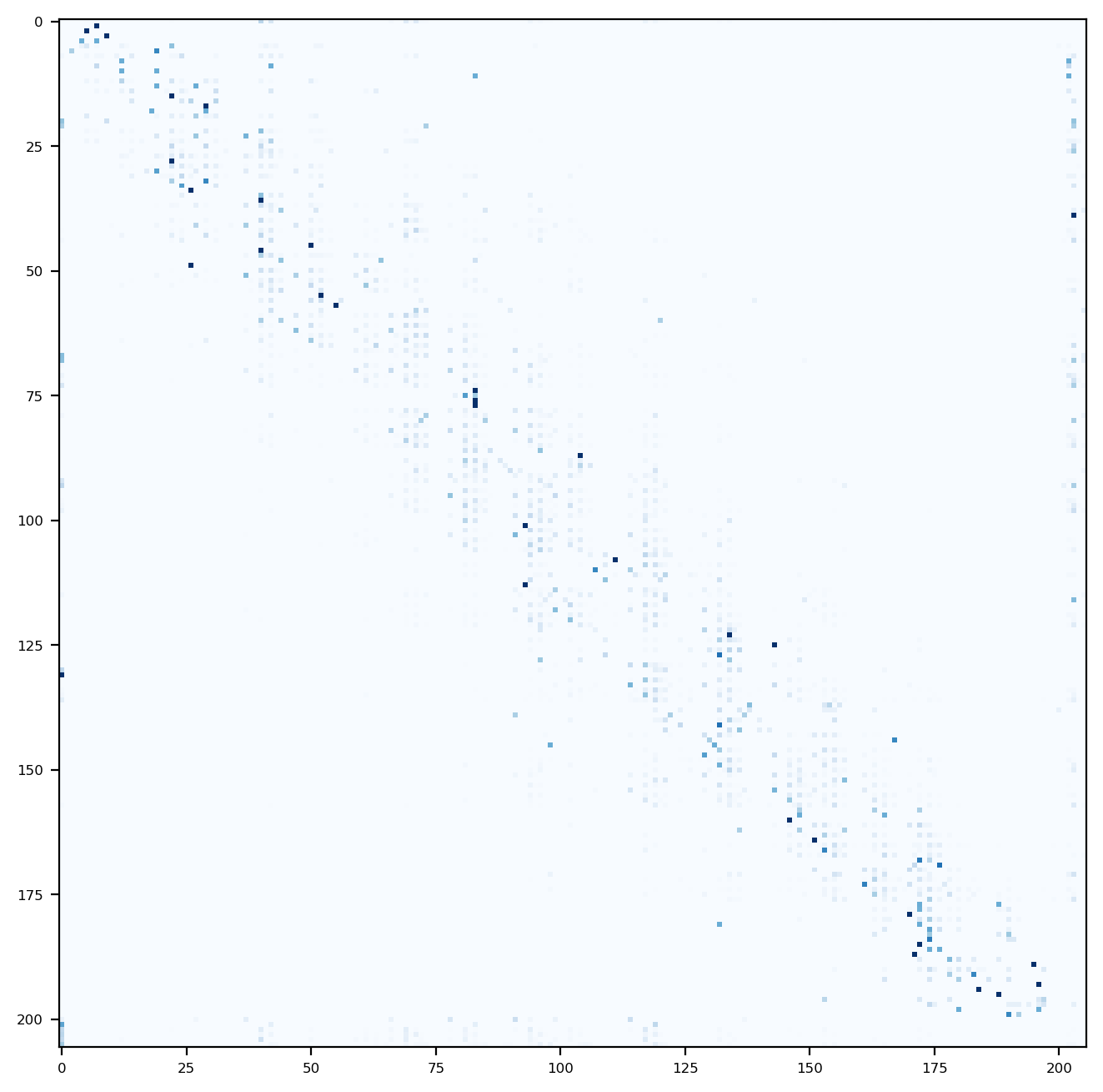
Plotting the probabilities reveals that \(\mathbf{P}\) is a rather sparse matrix containing many zeros. In fact, only approximately 7.86 percent of the entries are non-zero.
Sampling of New Melodies
Given the tensor P, we can generate new melodies using the function torch.multinomial which expects a probability (discrete) distribution.
I start with the terminal TERM_SYMBOL indicating the beginning and, when the second terminal is generated (which indicates the end), I terminate the generation.
generated_encoded_song = []
char = TERM_SYMBOL
while True:
    ix = torch.multinomial(P[stoi[char]],
        num_samples=1,
        replacement=True).item()
    char = itos[ix]
    if char == TERM_SYMBOL:
        break
    generated_encoded_song.append(char)
len(generated_encoded_song)
Let’s listen to some of the generated scores:
Negative Log Likelihood Loss.
The outcome is not particularly outstanding, but this is unsurprising given our very simple model. To evaluate the quality of our model, we can calculate the likelihood that our generative process produces for a specific training data point \(e_1, e_2, \ldots, e_k\), i.e.,
\[P(e_1) \cdot P(e_2 \ | \ e_1) \cdot \ldots \cdot P(e_{k-1} \ | \ e_k).\]We can add all the likelihoods (one for each data point) together and divide the sum by the number of data points. However, it is more convinient to use the negative log-likelihood since one can use addition.
log_likelyhood = 0.0
n = 0
for m in enc_songs:
    chs = [TERM_SYMBOL] + m + [TERM_SYMBOL]
    for ch1, ch2 in zip(chs, chs[1:]):
        ix1 = stoi[ch1]
        ix2 = stoi[ch2]
        prob = P[ix1, ix2]
        logprob = torch.log(prob)
        log_likelyhood += logprob
        n += 1

print(f'{log_likelyhood=}')
nll = -log_likelyhood
print(f'avg negative log likelyhood: {(nll/n)}')
This gives us a negative log-likelihood of approximately 2.6756.
The lower this value gets the better it is.
It can be no smaller than 0.
Feedforward Neural Network
One method of generating a melody using a feedforward network (FFN) is by addressing a classification task. Well, strictly speaking we do not even build a FFN, since there will be no activation function involved thus it is a linear model. However, from this starting point we could expand our model into a multi-layer perceptron (MLP). By avoiding the activation function, it is easier for me to explain exactly what is going on.
If we think in terms of classification a sequence of note should be classified as some successor note. So let us assume \(t\) consecutive notes are given then our aim is to identify the note that this sequence “represents”. For simplicity, I assume we only want to predict the next note given the previous one, that is, \(t=1\) holds. This stipulation means we won’t require substantial modifications compared to our previous approach.
Since our training process will be more computationally intensive than merely computing frequencies, it’s advisable to use hardware accelerators, if available. This can result in faster training and inference times and lower energy costs. To check if hardware acceleration is available, I employ the following code:
if torch.cuda.is_available():
    device = torch.device('cuda')
elif torch.backends.mps.is_available():
    device = torch.device('mps')
else:
    device = torch.device('cpu')

print(f'{device=}')
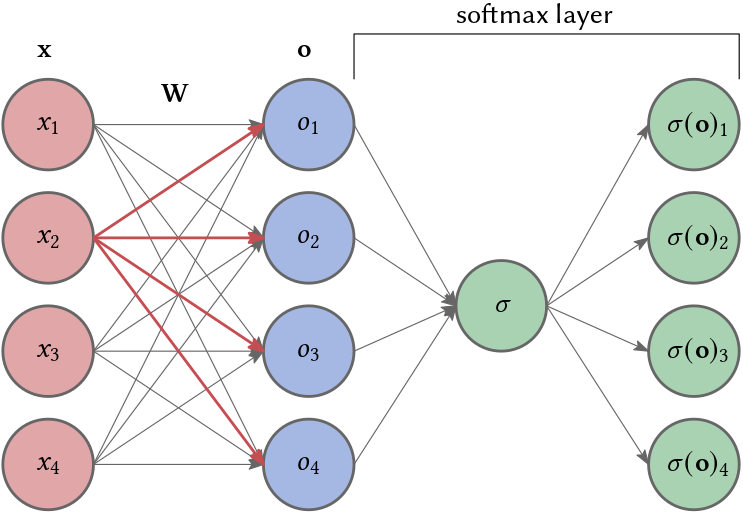
What we are going to implement is a fully-visible softmax belief network which only predicts the very next note given the previous note. However, instead of multiplying \(x_1\) to predict \(x_2\) via
\[h_{\theta}(x)_{j=1,\ldots,m} = \left(\alpha_0^{(j)} + \alpha_1^{(j)} \cdot x \right)_{j=1,\ldots,m},\]we do something similar but not quite the same. We hot-encode our alphabet \(\mathcal{X}\) of notes into
\[|\mathcal{X}| = m\]vectors \(\mathbf{x}_j = (x_1, \ldots, x_m)\), \(j=1, \ldots, m\) of length \(m\), such that,
\[h_{\theta}(\mathbf{x}_i)_{j=1,\ldots,m} = \left( w_{1}^{(j)} \cdot x_1 + w_{2}^{(j)} \cdot x_2 + \ldots + w_{m}^{(j)} \cdot x_m \right)_{j=1,\ldots,m} = \left( w_{i}^{(j)} x_i \right)_{j=1,\ldots,m}.\]In other words, we compute an embedding of our alphabet/domain of notes such that each note is encoded by an \(m\)-dimensional vector. This vector represents the probabilities of the next note. To transform these embeddings into probabilities we apply the softmax function. Our network is depicted in Fig. 2. Note that we do not use a bias term, i.e., there is no replacement for \(\alpha_0^{(j)}\).
Similar as before, our loss is the empirical mean of the negative log likelyhood
\[-\frac{1}{M} \sum_{i=1,j=y_i}^M \log(\sigma(\mathbf{o})_j),\]where \(j\) is the \(j^\text{th}\) note in our alphabet and \(y_i\), that is \((\mathbf{x}, y_j)\) is in our training data set.
Training Data Construction
Instead of calculating our probability matrix, I am going to generate labeled training data using the variables xs and ys (labels).
xs = []
ys = []
for m in enc_songs:
    chs = [TERM_SYMBOL] + m + [TERM_SYMBOL]
    for ch1, ch2 in zip(chs, chs[1:]):
        ix1 = stoi[ch1]
        ix2 = stoi[ch2]
        xs.append(ix1)
        ys.append(ix2)

xs = torch.tensor(xs, device=device)
ys = torch.tensor(ys, device=device)

# one-hot-encoding
xenc = F.one_hot(xs, num_classes=len(stoi)).float()
As mentioned, I employ a one-hot encoding for the input data.
That is, for encoding \(m\) unique elements one uses \(m\) unique \(m\)-dimensional vectors.
One component of these vectors is set to 1.0 and all others are 0.0.
F.one_hot assumes that our alphabet consists of whole numbers between 0 and \(m-1\), compare the documentation.
The \(i^{\text{th}}\) element is represented by a vetor where the \(i^{\text{th}}\) component is 1.0.
Note that our labels ys are not one-hot encoded.
Training
Next, I initialize a random matrix \(\mathbf{W} \in [-1;1]^{m \times m}\), or tensor, W with values ranging from -1.0 to 1.0.
This tensor includes our trainable parameters, which represent the single layer of our neural network.
W = torch.randn((len(stoi), len(stoi)), requires_grad=True, device=device)
Our network includes \(m\) inputs and outputs, with the softmax values of the outputs being interpreted as probabilities. Essentially, our “network” is just one large matrix!
The operation xenc @ W represents a matrix multiplication where xenc is an \(1700 \times m\) matrix and W is our \(m \times m\) matrix.
Here I use the power of parallel computation.
By employing probs[torch.arange(len(ys), device=device), ys], I address a single entry for each row.
Please note that probs[:, ys] does not work; instead of addressing a single entry, it addresses whole columns indexed by ys!
Also, be aware that I apply an unusually large learning rate.
# training aka gradient decent
epochs = 2_000
for k in range(epochs):
    # forward pass
    logits = xenc @ W
    odds = logits.exp()
    probs = odds / odds.sum(dim=1, keepdim=True)
    loss = -probs[torch.arange(len(ys), device=device), ys].log().mean()

    print(f'epoch {k}, loss: {loss.item()}')

    # backward pass
    W.grad = None # set gradients to zero
    loss.backward()

    # update
    W.data += -10.0 * W.grad
One iteration of the loop consist of the
- forward pass
- backward pass (backwardpropagation) done via
loss.backward()and - an update of our parameters done via
W.data += -10.0 * W.grad.
loss.backward() applies backpropagation thus computes the gradients and we can update W by
where \(\eta = 10\) is the learning rate.
After the initial 2000 epochs the loss is approximately 2.865.
This performance is somewhat inferior compared to the results achieved by our Markov chain.
However, by prolonging the training period, I managed to reduce the loss to around 2.707.
What is going on?
Let us assume we have only one sample \(\mathbf{x}\).
Forward Pass:
The forward pass starts with
\[\mathbf{o} = \mathbf{x} \cdot \mathbf{W}\]where \(\mathbf{x}\) is a one-hot encoded training data point. \(\mathbf{o}\) gets interpreted as (component-wise) logarithm of the odds
\[\mathbf{o} = \ln\left(\frac{\mathbf{p}}{\mathbf{1}-\mathbf{p}}\right)\]which is the logit, i.e., the inverse of the standard logistic function also called sigmoid. In fact, each data point in \(\mathbf{x}\) selects one row of \(\mathbf{W}\)
\[\mathbf{o} = \mathbf{x} \cdot \mathbf{W} = \begin{bmatrix} o_1 & o_2 & \ldots & o_m \end{bmatrix}.\]To compute “probabilities” we compute the softmax function (probs) of \(\mathbf{o}\), i.e.,
with
\[\sigma(\mathbf{o})_i = \frac{e^{o_i}}{\sum e^{o_j}}.\]Luckly the softmax has a simple derivative:
\[\frac{\partial \sigma(\mathbf{o})_i}{\partial o_j} = \begin{cases} \sigma(\mathbf{o}_k)_i - \sigma(\mathbf{o})_i^2 & \text{ if } i = j \\ -\sigma(\mathbf{o}_k)_i \sigma(\mathbf{o})_j & \text{ otherwise.} \end{cases}\]We can also compute the full Jacobian of the softmax vector-to-vector operation:
\[\nabla_{\mathbf{o}} \sigma = \mathbf{J}_{\mathbf{o}}(\sigma) = \begin{bmatrix} \sigma_1 - \sigma_1^2 & -\sigma_1 \sigma_2 & \ldots & - \sigma_1 \sigma_m \\ -\sigma_2 \sigma_1 & s_2 - \sigma_2^2 & \ldots & -\sigma_2 \sigma_m \\ \ldots & \ldots & \ldots & \ldots \\ -\sigma_m \sigma_1 & -\sigma_m \sigma_2 & \ldots & \sigma_m - \sigma_m^2 \end{bmatrix} = \text{diag}\left(\sigma\right) - \sigma^{\top} \sigma\]Similar then before, our loss $L$ is the mean negative log likelihood.
\[L(\mathbf{y}, \sigma) = -\sum\limits_{i=1}^{m} \log(s_i) = -\mathbf{y} \log(\sigma)^\top\]where \(\mathbf{y}\) is the one-hot encoded label vector, i.e.,
loss = -probs[torch.arange(len(ys), device=device), ys].log().mean().
Note that \(\mathbf{y}\) is a one-hot encoded vector, ys is not.
Backword Pass:
For the backpropagation we need
\[\nabla_{\mathbf{W}} L(\mathbf{y}, \sigma) = \nabla_{\mathbf{o}} L(\mathbf{y}, \sigma) \cdot \nabla_{\mathbf{W}} \mathbf{o}.\]Here we employ the chain rule. The sensitivity of cost \(L\) to the input to the softmax layer, \(\mathbf{o}\) is given by a gradient-Jacobian product, each of which we’ve already computed:
\[\begin{align} \nabla_{\mathbf{o}} L(\mathbf{y}, \sigma) &= -\nabla_{\mathbf{o}} \mathbf{y} \log(\sigma)^\top \\ &= -\mathbf{y} \nabla_{\mathbf{o}}\log(\sigma) \\ &= -\frac{\mathbf{y}}{\sigma} \nabla_{\mathbf{o}} \sigma \\ &= -\frac{\mathbf{y}}{\sigma} \cdot \mathbf{J}_{\mathbf{o}}(\sigma) \\ &= -\frac{\mathbf{y}}{\sigma} \cdot \left[ \text{diag}(\sigma) - \sigma^\top \sigma \right] \\ &= \frac{\mathbf{y}}{\sigma} \sigma^\top \sigma - \frac{\mathbf{y}}{\sigma} \text{diag}(\sigma) \\ &= \sigma - \mathbf{y}. \end{align}\]The \(\log\) and the devision operates component-wise and
\[\text{diag}\left(\sigma\right) = \begin{bmatrix} \sigma(\mathbf{o})_1 & 0 & \ldots & 0 \\ 0 & \sigma(\mathbf{o})_2 & \ldots & 0 \\ \ldots & \ldots & \ldots & \ldots \\ 0 & 0 & \ldots & \sigma(\mathbf{o})_m \end{bmatrix}\]holds. We have to apply the chain rule once again to finally get the desired update values for our weight matrix \(\mathbf{W}\):
\[\begin{align} \nabla_{\mathbf{W}} L(\mathbf{y}, \sigma) &= \nabla_{\mathbf{o}} L(\mathbf{y}, \sigma) \cdot \nabla_{\mathbf{W}} \mathbf{o} \\ &= (\sigma - \mathbf{y}) \cdot \nabla_{\mathbf{W}} (\mathbf{x} \cdot \mathbf{W})\\ &= (\sigma - \mathbf{y}) \cdot \mathbf{x}^{\top}. \end{align}\]Given that \(\sigma\) represents probabilities, and \(\mathbf{y}\) contains only zeros except for one instance of 1 at the position of the “correct” probability, the entries of the \(j^\text{th}\) row (\(x_j=1\)) of the gradient is \(p_i\) if the \(i^\text{th}\) probability is deemed “incorrect”, and \((p_i-1)\) otherwise. All other entries are zero. Note also that \(\mathbf{x}\) is also a one-hot encoded vector. Consequently, if a probability is correct, it gets increased by \(1-p_i\) and decreased by \(p_i-1\) otherwise. Therefore, probabilities that are more incorrect experience a larger increase or decrease.
We can actually check this result! Using the following code:
# use only 1 data point
xs = xs[:1]
ys = ys[:1]

# one-hot-encoding
xenc = F.one_hot(xs, num_classes=len(stoi)).float()

# reinitiate W
W = torch.randn((len(stoi), len(stoi)), requires_grad=True, device=device)

logits = xenc @ W
counts = logits.exp()
probs = counts / counts.sum(dim=1, keepdim=True)
loss = -probs[torch.arange(len(ys), device=device), ys].log().mean()

# backward pass
W.grad = None
loss.backward()
y = torch.zeros(len(stoi), device=device)
y[ys[0]] = 1
print(W.grad) # same
print(xenc.T @ (probs-y)) # same
print(W.grad == xenc.T @ (probs-y)) # all true
Batching:
So far we only considered the math using a single data point \(\mathbf{x}\). Let us consider a batch of points, i.e.,
\[\mathbf{O} = \mathbf{X}\mathbf{W} = \begin{bmatrix} \mathbf{x}_1 \\ \mathbf{x}_2 \\ \vdots \\ \mathbf{x}_n \end{bmatrix} \mathbf{W}\]The softmax is still a vector-to-vector transformation, but it’s applied independently to each row of $\mathbf{X}$:
\[\mathbf{S} = \begin{bmatrix} \sigma(\mathbf{o}_1) \\ \sigma(\mathbf{o}_2) \\ \vdots \\ \sigma(\mathbf{o}_n) \end{bmatrix}\]We can do the exact same steps but I will skip this part. For the interested reader I refer to
Important is that
\[\mathbf{J}_\mathbf{O}(L) = \mathbf{J}_\mathbf{S}(L) \mathbf{J}_\mathbf{O}(S) = \frac{1}{n} \left( \mathbf{S} - \mathbf{Y} \right)\]and
\[\mathbf{J}_\mathbf{W}(L) = \mathbf{J}_\mathbf{S}(L) \mathbf{J}_\mathbf{O}(S) \mathbf{J}_\mathbf{W}(O) = \frac{1}{n} \left( \mathbf{S} - \mathbf{Y} \right) \mathbf{X}.\]We can also check this result:
# one-hot-encoding
xenc = F.one_hot(xs, num_classes=len(stoi)).float()

# reinitiate W
W = torch.randn((len(stoi), len(stoi)), requires_grad=True, device=device)

logits = xenc @ W
counts = logits.exp()
probs = counts / counts.sum(dim=1, keepdim=True)
loss = -probs[torch.arange(len(ys), device=device), ys].log().mean()

# backward pass
W.grad = None
loss.backward()
y = torch.zeros((len(ys), len(stoi)), device=device)
y[torch.arange(len(ys), device=device),ys] = 1

print(W.grad) # same
print(xenc.T @ (probs-y)/len(ys)) # same
print(torch.allclose(W.grad, xenc.T @ (probs-y)/len(ys))) # true
Further Considerations
Now, the natural question is: what is the best possible performance we could achieve?
The answer is that we should aim to match the performance of the Markov chain.
Indeed, as the process continues, we should expect that the matrix W will gradually converge towards P.
Moreover, we should not anticipate surpassing the results achieved by our Markov chain even if we deepen our network, that is, by introducing some hidden layers. A very good example of useful informations are described in (Johnson, 2017), I discussed in Part I of this series. For instance, Johnson adds (compare his interesting Blog post)
- Positional: note within the score (that is what we use)
- Pitchclass: one of the twelve classes
- Previous vicinity: surrounding notes where played or aticulated last timestep (only useful for polyphonic music)
- Previous context: the amount of C’s, A’s and so on are played the last timestep (only useful for polyphonic music)
- Beat: a binary representation of position within the measure
However, our expectations may shift if we modify the input, referring to the data that the network processes.
That being said, we could enhance the training duration.
For instance, introducing a hidden layer results in a loss of 2.693 after 2000 epochs.
W1 = torch.randn((len(stoi), len(stoi)//4),
                 requires_grad=True, device=device)
W2 = torch.randn((len(stoi)//4, len(stoi)),
                 requires_grad=True, device=device)
epochs = 2_000
for k in range(epochs):
    # forward pass
    x = xenc @ W1
    logits = x @ W2
    odds = logits.exp()
    probs = odds / odds.sum(dim=1, keepdim=True)
    loss = -probs[torch.arange(len(ys), device=device), ys].log().mean()

    print(f'epoch {k}, loss: {loss.item()}')

    # backward pass
    W1.grad = None # set gradients to zero
    W2.grad = None # set gradients to zero
    loss.backward()

    # update
    W1.data += -10.0 * W1.grad
    W2.data += -10.0 * W2.grad
References
- Oore, S., Simon, I., Dieleman, S., Eck, D., & Simonyan, K. (2018). This time with feeling: Learning expressive musical performance.
- Johnson, D. D. (2017). Generating polyphonic music using tied parallel networks. EvoMUSART.