Musical Interrogation I - Intro
This article is Part 1 in a 4-Part Series.
- Part 1 - Musical Interrogation I - Intro
- Part 2 - Musical Interrogation II - MC and FFN
- Part 3 - Musical Interrogation III - LSTM
- Part 4 - Musical Interrogation IV - Transformer
Whereas the human mind, conscious of its conceived purpose, approaches even an artificial system with a selective attitude and so becomes aware of only the preconceived implications of the system, the computers would show the total of available content. Revealing far more than only the tendencies of the human mind, this nonselective picture of the mind-created system should be of significant importance. – Gerbert Brün (1970)
In this series of posts, I will talk about melody generation using machine learning. I start by reflecting on computer music. Furthermore, I give a short and selective overview of some techniques to generate melodies that captured my interest, focusing on recurrent neural networks (RNN) to generate monophonic melodies for now.
I intend to build an interactive system that facilitates the musical dialog between humans and machines. In the end, a user should be able to interrogate the machine learning model such that an evaluation of the model’s ability is possible and maybe – a big maybe – users can enhance their creative process.
Reflection on Computer Music
Due to the recent advances in machine learning, especially in the domain of deep learning, computer music is regaining attraction. What started in the early 1960th, when rule-based methods such as Markov chains, hidden Markov models (HMM), generative grammars, chaotic systems, and cellular automata were applied to generate musical compositions, slowed down over the years. Of course, since then, computers have always accompanied music production, but algorithms have taken a backseat when it comes to the structure of music itself. Today, a reinvigoration of computer music might happen, but what will be at the forefront? The algorithm? The artist? Or a massive amount of data?
In his book Algorithmic Composition: Paradigms of Automated Music Generation (Nierhaus, 2009) Gerhard Nierhaus makes an essential distinction between genuine composition and style imitation. This terminology can bring nuances into the discussion around machines, algorithms, and data replacing human creativity.
Style imitation is more applicable when music is not the main focus of interest but amplifies or accompanies something else, e.g., ads, computer games, or movies. In a computer game, you want music that captures the dynamic situation of the game; thus, surprises are undesirable.
Genuine composition appeals more to the artist who wants to play, experiment, and break things or criticize narratives. Genuine composition seduces the audience’s desire for experimentation, confrontation, and reflection on something new and unexpected.
While genuine composition carries much novelty, style imitation can be categorized into a set of preexisting styles of musical compositions. The results generated by different techniques lean more or less towards one or the other. For example, compositions generated by Markov chains (see Probabilistic Melody Modeling) lean more towards style imitation since the model samples from a learned distribution to estimate the structure of a particular composition. On the other hand, using cellular automata is a technique more suited for genuine composition because no learning is involved. Instead, cellular automata are dynamic systems capable of complex emergent behavior that can not be explained by solely looking at the parts of the system. Of course, there is no black and white. Instead, each composition or technique lives on a spectrum, and it might be impossible to decide where exactly. If a machine learning model learns some non-obvious high-level structure, i.e., a probability distribution, from its training data, does this yield novelty or not? It depends, I guess.
However, this “problem” is old, isn’t it? Looking at the history of classical Western music, there are moments in time when it seemed that nothing was left to say and style imitation was inevitable. For example, after one of the most quintessential romantic composers, Richard Wagner, there were view possibilities left concerning tonal music. Consequently, the need for more chromaticism and dissonance was unavoidable, leading to the extreme case of Schönberg’s atonal compositions.
Concerning artificial intelligence, our current century is an era of deep learning models for which model size, data, parameters, and training time are more important than the underlying algorithm. These models can combine, alter, and re-synthesis music from recorded history. This re-combination and alteration seem similar to human composers’ working process, which is primed by their environment, education, and culture. There is no doubt that these models can create music via style imitation but how good are they regarding genuine composition? Is not learning from existing data style imitation per definition? Well, again, even if all the data is known, one can argue that there are hidden high-level structures within the data that we are entirely unaware of. A prime example is discovering a new way to multiply small matrices found via reinforcement learning (Fawzi et al., 2022).
If machines, revealing these structures, are creative is a question that can hardly be answered objectively, but, after all, the question might not be of great interest. I instead look at the human condition and ask what such machines mean for our being in the world. And here, we can say that if we do not try to understand our new black boxes, we rob ourselves of the experience of understanding, which, I think, is a fundamental desire. But at the same time, if we do not give up understanding but enhance it with machine power (seen as a tool), the reverse can be true. Beyond a lack of understanding, the lack of experienced practice is the more obvious loss we suffer. The uncomfortable mood I sometimes develop when the achievements of AI shimmer through my perception comes from a fear of losing my habituated being in the world. I ask myself: will machines write my code? Will I lose the enjoyment that I get out of coding? Will I lose my identity as a programmer? However, this loss has more to do with technology and economics. We think of technology as a natural evolutionary force that points towards a better future. And due to economic necessities, we have to adapt to stay productive. However, without the industrial revolution, I would never have been able to enjoy programming in the first place. Therefore, fear and excitement are reasonable reactions to this time of disruption.
But let’s come back and go back to the actual topic. One of the challenges AI researchers face today is not so much the generation of novelty but the evaluation of it, especially in the case of aesthetics, which is somewhat subjective. Within the generative process, the machine has to “judge” if the piece is engaging. Otherwise, the whole process is nothing more than a sophisticated but impracticable random search through the space of all possible compositions. However, interest depends on the cultural context. Maybe Schönberg’s atonal, thus ungodly music, would not have attracted anybody in the 13th century. Judging if novelty is sensible seems to require an embodiment in the world. Therefore, as an art form, I find fully automated opaque music-generating systems that lack human interaction undesirable because they, in the end, lead to a mode of passive consumption. Instead, human intelligence is needed to bring intentionality into the composition. I imagine an interconnected relationship where artificial communication guides humans and machines to new places.
Even though machines are still unable to develop intentionality of their own, composing is a partially rigorous and formal endeavor; thus, algorithms and machines can certainly help with realizing intentions. Contrary to popular belief, music and computer science / mathematics are much more related than they seem. And there is no reason to believe that algorithms can not only be aesthetically and intellectually beautiful but can also evoke emotions.
However, computer music is diverse, and as an amateur, I should be careful in my assessment. I encountered rule-centered computer music, highly interactive live programming (which is also a movement), real-time music generation, sonification, and data-centered computer music. While rule-centered music generation is transparent and offers low-level control, data-centered generation is often opaque and offers only high-level control, at least, up to this date. Live programming is highly interactive and relies on real-time communication between performer and audience as well as real-time artificial communication between performer and machine.
Communication between humans and machines excites me the most since it offers the possibility to reflect on algorithms, programs, machines, data, and technology in general. It goes beyond analytical contemplation by making algorithms experiencable. Furthermore, learning from human feedback to calibrate generative models such that they represent our experienced ups and downs, twists and turns in music by injecting intentionality in order to steer generative models might be the way to go. The term co-pilot comes to mind.
Melody Generation
For the interested reader, the survey AI Methods in Algorithmic Composition: A Comprehensive Survey (Rodriguez & Vico, 2014) and A Comprehensive Survey on Deep Music Generation: Multi-level Representations, Algorithms, Evaluations, and Future Directions (Ji et al., 2020) offer an excellent first overview of the different techniques up to the year 2014 and 2020, respectively.
A Difficult Problem
Let us first reflect on the question of why melody generation is tricky. First of all, in music, intervals are everything. It does not matter so much if one plays a C or B; what matters is the relation of notes within a piece, i.e., playing A-C or A-B. Intervals are so ingrained into music that musicians give them certain names such as minor third, perfect fifth, or tritone (the Devil’s tone). It is no coincidence that major and minor chords, as well as most scales, are asymmetrical because it gives each note a distinctive quality within a chord or a scale.
In addition, this relation is multi-dimensional. We have melody, i.e., playing note after note horizontally, and harmony, i.e., vertical relations, for which we play notes together (chords). On top of that, what happens in measure 5 may directly influence what happens in measure 55, without necessarily affecting any of the intervening material. These relations can be all over the place and span a very long sequence! Good music hits a sweet spot between repetition and surprise, and landing on that spot is quite challenging. Together, these properties make melody (or polyphonic) generation hard.
The Music Generation Process
Many artists and researchers took on the challenge, and machine learning techniques increasingly play an essential role. The learning and generation are based on two major categories of representations: either symbolic notation or performed pieces of music.
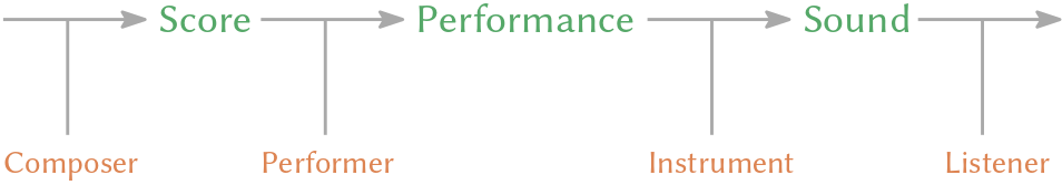
Classical music and most other kinds of music as we know them came into being through the music generation process depicted in Figure 1. Composers write a score that leads to the performing musicians (the execution of the score) who are exciting their instruments. This excitement causes the instrument to vibrate, and due to its physicality, it pushes air molecules around. Molecules bump into each other in some areas and tend to leave other areas—a displacement we call wave. In principle, the energy of the excitement travels outwards through the air to the listener’s ear. The information gets more and more concrete. While a score is an abstract representation, the sound caused by instruments is very concrete. It is, in fact, so concrete that it is different for every listener since each of us perceives sound slightly differently.
Abstraction removes us from the messy reality and enables communication, but it also conceals the singularity of beings. Concerning melody generation we have to ask how much abstraction is justified. A score represented by a note sheet without any information about the dynamics is “more” symbolic or abstract than a note sheet that contains hints for the tempo and loudness. Raw audio material is far away from the much more abstract symbolic notation and a lived thorough performance is a singular event.
Using symbolic notation is more accessible, but one loses the slight variations, dynamics, and other qualities that make the result feel so humanly made. However, composers who want to use melody generation to support their process might be happy to introduce these qualities by themselves. It is a question of application. The same is true for the mono- and polyphonic generations. Do we want to generate a full-fetched performance, a melody snippet (monophonic), or something in between? In this blog post, I will focus on the monophonic generation (one note at a time).
Autoregressive Generative Models
An autoregressive (AR) model is a representation of a type of random process that specifies that the output variable depends linearly on its own previous values and on a stochastic term (an imperfectly predictable term). In the field of machine learning these models are sequence generative models, that is, they learn an approximation of the real probability distribution.
Let’s assume we are given access to a dataset \(\mathcal{D} \subseteq \mathcal{X}^n\) of \(n\)-dimensional datapoints \(\mathbf{x}\). Each datapoint represents a sequence of events—in our case a sequence of notes. By the chain rule of probability, we can factorize the joint distribution over the \(n\)-dimensions as
\[P(\mathbf{x}) = \prod_{i=1}^n P(x_i | x_1, x_2, \ldots, x_{i-1}) = \prod_{i=1}^n P(x_i|\mathbf{x}_{<i}),\]where
\[P(x_i | x_1) = P(x_i | X_1 = x_1) \text{ and } \mathbf{x}_{<i} = (x_1, x_2, \ldots, x_{i-1}).\]If we allow every conditional \(P(x_i|\mathbf{x}_{<i})\) to be specified in a tabular form, then such a representation is fully general and can represent any possible distribution over \(n\) random variables. However, the space complexity for such a representation grows exponentially with \(n\).
In an autoregressive generative model, the conditionals are specified as parameterized functions (hypothesis) with a fixed number of parameters
\[P_{\theta_{i}}(x_i|\mathbf{x}_{<i}) = h_i(x_1, x_2, \ldots, x_{i-1}),\]where \(\theta_{i}\) denotes the set of parameters used to specify the mean function
\[h_{\theta_{i}} : \mathcal{X}^{i-1} \rightarrow [0;1]^{|\mathcal{X}|},\]with the condition that the \(\|\mathcal{X}\|\) probabilities sum up to 1. The number of parameters of such a model is given by
\[\sum_{i=1}^n |\theta_{i}|.\]Linear Models
Suppose
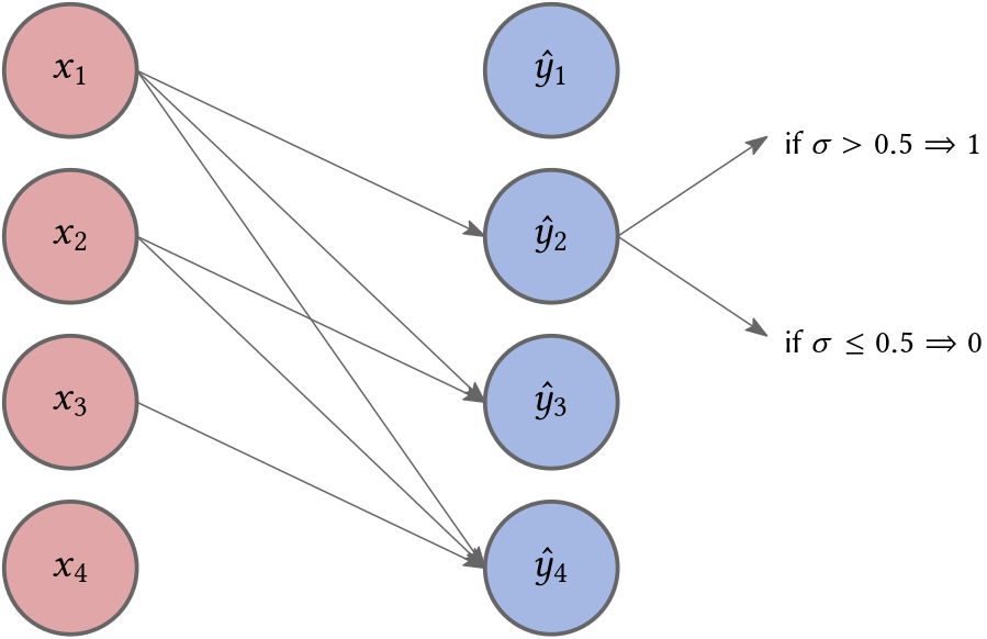
\[\mathcal{X} = \{0,1\} \quad \text{ (Bernoulli random variables)}\]then a very simple model would be a linear combination of the input elements followed by a sigmoid non-linearity (to restrict the output to lie between 0 and 1):
\[h_{\theta_{i}}(x_1, x_2, \ldots, x_{i-1}) = \sigma\left( \alpha_0^{(i)} + \alpha_1^{(i)} x_1 + \ldots + \alpha_{i-1}^{(i)} x_{i-1} \right),\]where
\[\sigma(x) = \frac{1}{1+e^{-x}}\]and
\[\theta_i = \{\alpha_0^{(i)}, \alpha_1^{(i)}, \ldots, \alpha_{i-1}^{(i)}\}\]denote the parameters of the mean function. Note that this simple model has \(\mathcal{O}(n^2)\) parameters (instead of the \(\mathcal{O}(2^{n-1})\)) required if we use a tabular representation for the conditionals. In Fig. 2
\[\hat{y}_i \in \mathcal{X} \text{ is } 1 \text{ if } h_{\theta_{i}}(x_1, x_2, \ldots, x_{i-1}) > 0.5,\]otherwise it is 0.
In the general case, where \(|\mathcal{X}| = m\), i.e. it consists of a finite number of possible events—in our case notes—a linear model should output $m$ numbers between 0 and 1 that sum up to 1. In that case, \(h_{\theta_{i}}(x_1, x_2, \ldots, x_{i-1})\) outputs an \(m\)-dimensional vector
\[\mathbf{p}_i = (p_{i1}, p_{i2}, \ldots, p_{im})\]where
\[p_{ij} = \frac{e^{z_{ij}}}{\sum_{k=1}^m e^{z_{ik}}} = \sigma(\mathbf{z}_{i})\]with
\[z_{ij} = \alpha_0^{(i,j)} + \alpha_1^{(i,j)} x_1 + \ldots + \alpha_{i-1}^{(i,j)} x_{i-1}.\]Thus we replace the sigmoid by softmax and we would require \(\mathcal{O}(n^2 \cdot m)\) parameters.
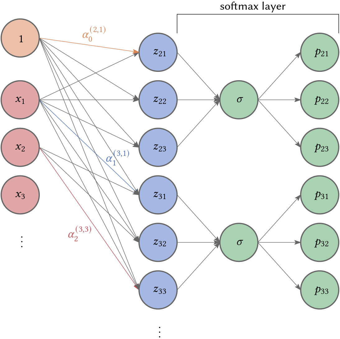
We can express this via a matrix-vector multiplication
\[\mathbf{z}_{i} = \mathbf{A}_i \mathbf{x}_{<i} + \mathbf{b}_i,\]where
\[\mathbf{A}_{i} = \begin{bmatrix} \alpha_1^{(i,1)} & \alpha_2^{(i,1)} & \ldots & \alpha_{m-1}^{(i,1)} \\ \alpha_1^{(i,2)} & \alpha_2^{(i,2)} & \ldots & \alpha_{m-1}^{(i,2)} \\ \vdots & \vdots & \vdots & \vdots \\ \alpha_1^{(i,m)} & \alpha_2^{(i,2)} & \ldots & \alpha_{m-1}^{(i,m)} \end{bmatrix}, \quad \mathbf{b}_i = \begin{bmatrix} \alpha_0^{(i,1)} \\ \alpha_1^{(i,2)} \\ \vdots \\ \alpha_0^{(i,m)} \end{bmatrix}.\]For example, if we have three events \(m=3\) (see Fig. 3) and \(n=5\) then
\[\mathbf{A}_{5} = \begin{bmatrix} \alpha_1^{(3,1)} & \alpha_2^{(3,1)} & \alpha_3^{(3,1)} & \alpha_4^{(3,1)}\\ \alpha_1^{(3,2)} & \alpha_2^{(3,2)} & \alpha_3^{(3,2)} & \alpha_4^{(3,1)}\\ \alpha_1^{(3,3)} & \alpha_2^{(3,3)} & \alpha_3^{(3,3)} & \alpha_4^{(3,1)} \end{bmatrix}, \quad \mathbf{A}_{3} = \begin{bmatrix} \alpha_1^{(2,1)} & \alpha_2^{(2,1)} \\ \alpha_1^{(2,2)} & \alpha_2^{(2,2)} \\ \alpha_1^{(2,3)} & \alpha_2^{(2,2)} \end{bmatrix}.\]Note that if we only want to compute the next note of a melody given a sequence of $n-1$ notes, we are only interested in
\[P(x_n|x_1,x_2,\ldots, x_{n-1}).\]Thus, our network can be much simpler, i.e., we only need to compute
\[z_n = \mathbf{A}_n \mathbf{x}_{i<n} + \mathbf{b}_n.\]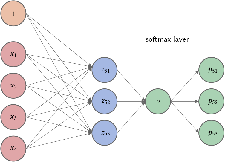
We could share our parameters for computing the next note for a sequence shorter than \(n-1\) notes by seting
\[x_j = 0 \text{ for } j \geq i.\]This architecture is often called neural autoregressive density estimator. By sharing, we reduces the amount of parameters to \(\mathcal{O}(n \cdot m)\). We will use such a feedforward neural network (without a bias term and assuming \(n=2\)) in Part II - FNN of this series.
Multi-Layer Perceptrons
A natural way to increase the expressiveness of an autoregressive generative model is to use more flexible parameterizations for the mean function (our hypotheses), e.g., multi-layer perceptrons (MLP). For example, consider the case of a neural network with 1 hidden layer. The mean function for variable $i$ can be expressed as
\[\begin{array} \mathbf{h}_i &= \sigma\left(\mathbf{W}_i \mathbf{x}_{< i} + \mathbf{c}_i \right) & \quad \text{ (component-wise sigmoid)}\\ \mathbf{z}_i &= \sigma\left( \mathbf{A}_{i} \mathbf{h}_i + \mathbf{b}_i \right) & \quad \text{ (softmax)} \end{array}\]where \(\mathbf{h}_i \in \mathbb{R}^d\) denotes the hidden layer activations for the MLP and
\[\theta_i = \{ \mathbf{W}_i \in \mathbb{R}^{d \times (i-1)}, \mathbf{c}_i \in \mathbb{R}^d, \mathbf{A}_{i} \in \mathbb{R}^{(i-1) \times d}, b_i \in \mathbb{R}^m \}.\]are the set of parameters for the mean function. Note that if $d$ is small the information gets compressed. The total number of parameters in this model is in \(\mathcal{O}(n^2 \cdot d)\) and is dominated by the matrices. Sharing both types of matrices reduces the complexity to \(\mathcal{O}(n \cdot d)\)
\[\theta = \{ \mathbf{W}_n \in \mathbb{R}^{d \times (n-1)}, \mathbf{c}_n \in \mathbb{R}^d, \mathbf{A}_n \in \mathbb{R}^{(n-1) \times d}, \mathbf{b}_n \in \mathbb{R}^m \}.\]computing
\[\begin{array} \mathbf{h}_i &= \sigma\left(\mathbf{W}_n \mathbf{x}_{< n} + \mathbf{c}_n \right) & \quad \text{ (component-wise sigmoid)}\\ \mathbf{z}_n &= \sigma\left( \mathbf{A}_n \mathbf{h}_n + \mathbf{b}_n \right) & \quad \text{ (softmax)} \end{array}\]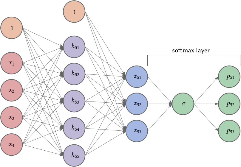
Discrete Markov Models
In my post Probabilistic Melody Modeling, I used a (discrete) first-order Markov chain (MC) (also called Markov process) to generate melodies after learning the model from one piece of music. The approach was simple: translate the frequency of note transitions into probabilities. For example, if the piece is defined by the note sequence A-B-B-A-C-A-B and the duration of each note is the same, then
\[P(X_{t+1} = B \ | \ X_{t} = A) = \frac{2}{3}, \quad P(X_{t+1} = C \ | \ X_{t} = A) = 1.0.\]To determine which note comes next, we only look at the previous note, i.e. at a very narrow context. Using a first-order Markov model, one would estimate the probability of the melody (not considering note duration) A-B-F by
\[P(X_0 = A) \cdot P(X_1 = B \ | \ X_0 = A) \cdot P(X_2 = F \ | \ X_1 = B).\]Using our notation above this corresponds to very simple hypotheses
\[h_{\theta_{i}}(x_{i-1}) = \left( c_1, \ldots, c_m \right) = \left( \hat{P}(X_{i} = x_1|X_{i-1} = x_{i-1}), \ldots, \hat{P}(X_{i} = x_m|X_{i-1} = x_{i-1}) \right),\]where $m$ is the number of possibly accoring notes and
\[\hat{P}(X_i = x_i|X_{i-1} = x_{i-1})\]is the empirical probability of \(x_i\) accuring after \(x_{i-1}\), i.e. the frequency of this event. In this example, a state is defined by a note, e.g. A.
Hidden Markov models (HMM) are Markov chains with hidden states. There are also a finite number of states, probabilistic transitions between these states, and the next state is determined by the current state, but we are unsure in which state the process is currently in. The current hidden state \(Z_t\) emits an observation \(X_t\). In other words, instead of going from one observed variable to the next, e.g., one note to the next, we move from one distribution of observations to the next, e.g. from one distribution of notes to the next!
For example, imagine a prisoner who has to estimate the outside weather (hidden state) by observing the dirt on the guard’s boots (emissions). If he knows all the probability transitions (e.g., from sunny to rainy, sunny to dirty on boots, etc.) and existing states, the prisoner could model the problem by an HMM, compare Figure 4.
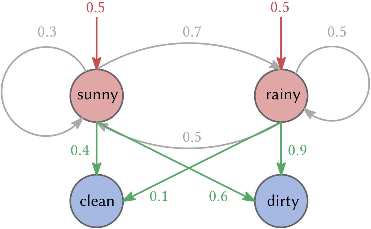
The prisoner could ask: given the HMM and an observation sequence \(X_0, \ldots, X_n\), what is the likelihood that this sequence occurs (likelihood problem)? One could also ask: what are the hidden states \(Z_0, \ldots, Z_n\) that “best” explains the observations (decoding problem). Moreover, what we are more interested in is: given an observation sequence \(X_0, \ldots, X_n\), learn the model parameters \(\theta\) that maximizes the likelihood for our observation (learning problem)! Similar to neural networks, one defines the architecture of the HMM (states and transitions), then solve the learning problem and infer new melodies from the learned HMM. In music, hidden states often lack interpretability. Therefore, it needs to be clarified which architecture one should choose.
HMM is a special case of dynamic Bayesian networks where a single hidden state variable represents the entire state of the world. With respect to music, using hidden Markov models we can model more abstract states that we can not directly observe, for example,
Using higher-order MC or HMM widens the context to multiple notes of the past. For our MC example A-B-F this would mean the probability changes to
\[P(X_0 = A) \cdot P(X_1 = B \ | \ X_0 = A) \cdot P(X_2 = F \ | \ X_0 = A \ \land \ X_1 = B).\]But due to the chain property (linearity), this does not necessarily lead to better results since widening the range leads very quickly to overfitting, i.e., the model reproduces more or less exact replica because it does not generalize—more is not always better. In any case, the learning stays stepwise causal, i.e., one note after the other without jumping around. By focusing on linear temporal dependencies, these models need to take into account the higher-level structure and semantics important to music. By model design, HMMs have very limited memory and are thus also incapable of modeling the longer term structure that occurs in original musical pieces.
Their applications in musical structure generation goes back to Harry F. Olson around 1950, and in 1955, the first machine produced Markov models of first and second order in regard to pitches and rhythm (Nierhaus, 2009). In (Van Der Merwe & Schulze, 2011), the authors used first-, higher-, or mixed-order MCs to represent chord duration, chord progression, and rhythm progression and first-, higher-, or mixed-order HMM to describe melodic arc.
A more rigorous and recent discussion, including polyphonic generation, be found in (Collins et al., 2016).
Long-term Memory?
As stated, the challenge is primarily due to long-term relations. One way of tackling this issue is to increase the memorizing capability of the model. With this in mind, looking at the catalog of model types within the field of deep learning one can spot multiple alternatives to Markov chains for melody generation.
One obvious choice is the long short-term memory recurrent neural networks (LSTM) (Hochreiter & Schmidhuber, 1997), a type of recurrent neural network (RNN) that allows information to persist for a longer time by letting it flow almost directly through time.
In theory, vanilla RNNs can learn the temporal structure of any signal, but due to computational reasons (vanishing/exploding gradients), they can not keep track of temporally distant events. If you want to learn more about RNNs, I highly recommend the blog article The Unreasonable Effectiveness of Neural Networks by Andrej Karpathy. In his blog post, he writes:
RNNs combine the input vector with their state vector with a fixed (but learned) function to produce a new state vector. This can, in programming terms, be interpreted as running a fixed program with certain inputs and some internal variables. – Andrej Karpathy
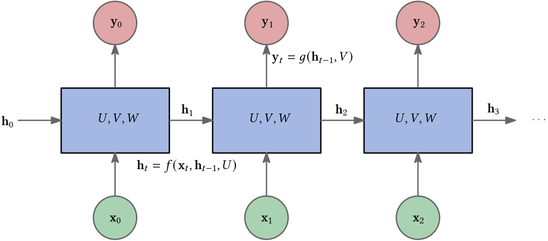
RNNs are similar to multilayered perceptrons (MLPs) but allow for connections from the output of one unit into the input of another unit located at a shallower layer than itself, i.e., closer to the input of the network. The information no longer flows acyclic through the network. Instead, recurrent feedback is introduced and allows an RNN to take into account its past inputs together with new inputs. Essentially, an RNN predicts a sequence of symbols given an input sequence. But using an RNN is like writing a thousand letters on the same piece of paper and then figuring out the information contained in the first letter—it is a mess; the information gets washed away. In Figure 5 the basic components of an RNN are depicted. Using my analogy, the piece of paper are the matrices $U,V,W$ which are learnable parameters. They are shared through time!
The extension, motivated by the shortcomings of vanilla RNNs, are LSTM RNNs or just LSTMs. LSTMs learn which information they should keep in long-term memory and which information they can forget after a short period. Instead of just writing all the letters on the piece of paper, we use our rubber and get rid of some writings while highlighting other passages.
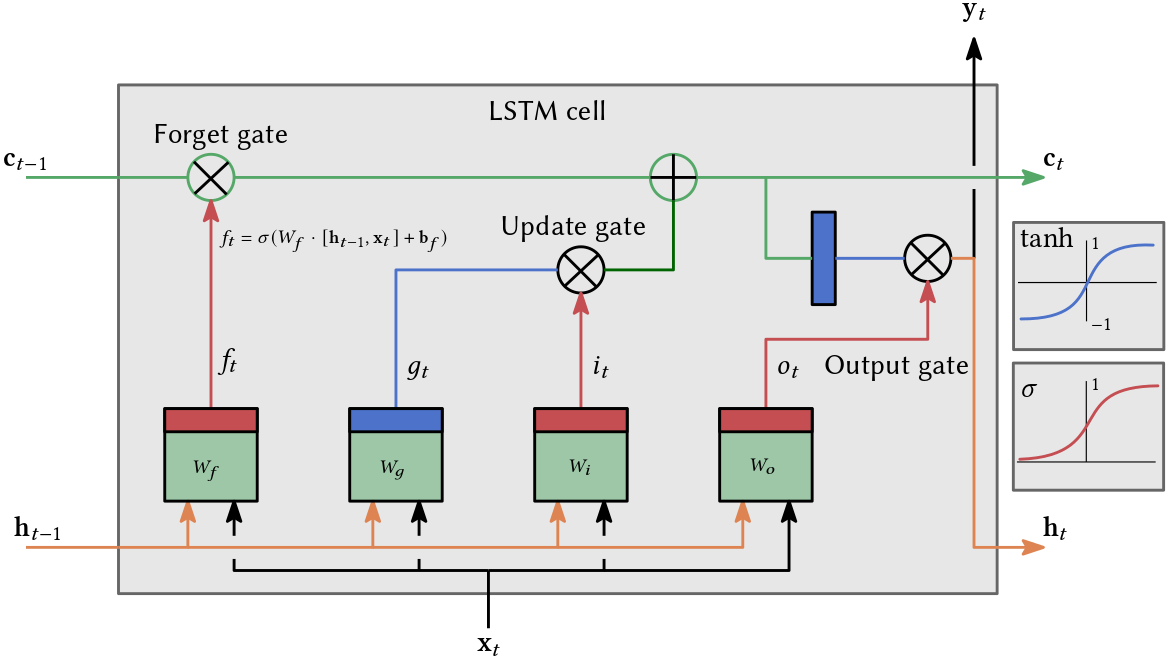
There is plenty of good material which explains LSTMs much more accurately than I can ever do. Figure 6 shows a sketch of a very complicated-looking LSTM cell where each green square is a linear transformation, each red bar indicates a sigmoid activation, and blue bars indicate a tanh activation. All the sigmoid activations are used to control the memorizing strategy (rubber and highlighter). First, the cell “decides” what to keep in the long-term state \(\mathbf{c}\_{t-1}\) via \(f_t\).
Then $i_t$ decides what to add to the long-term state. In addition, $o_t$ decides what part of the new long-term state will make up the short-term state \(\mathbf{h}_t.\) The importance is that along the path from \(\mathbf{c}_{t-1}\) to \(\mathbf{c}\_{t},\) there is only a simple multiplication and addition! Therefore, information can persist for longer.
Note, however, that LSTMs can still access information of time step \(t\) only via time step \(t-1\). There is no direct access to information compared to the attention mechanism (Bahdanau et al., 2014), and the transformer (Vaswani et al., 2017), which led to the most recent breakthroughs in the field of deep learning. Just a few days ago, another RNN, called RWKV-LM, claimed to achieve similar results; thus, the last word has yet to be spoken.
Application of Recurrent Neural Networks
In (Todd, 1989) Peter M. Todd used a vanilla RNN to generate melodies. Various issues are discussed in designing the network. Note that at this time in the young history of machine learning, there were no user-friendly software libraries available, and there was much more thinking going on in designing the network on a fine-grained level. The author also suggests using multi-layered perceptrons (MLPs) by explicitly modeling time and either showing the whole piece to the network or using a sliding-window approach, e.g., showing one bar at a time and predicting the next bar. In the end, Todd uses an RNN with 15 hidden units and 15 output units (1 note-begin unit and 14 pitch units) trained for 8500 epochs (cycle through the entire training set) using a handful of sliced melodies. Fewer hidden units led to more training. By today’s standard, Todd’s network was tiny. Todd assumes the key of C from D4 to C6. The note-begin unit indicates if the note begins or it merely continues. Interestingly, Todd discusses a pitch-interval representation. Instead of outputting the actual pitch values, the network outputs the relative transitions (intervals/pitch changes) in semitones. For example, instead of A-B-C the network outputs A-(+1)-(-3). The advantage is that outputs are more key-independent and can range over an extensive range of notes even if there are only view output units. This allows for the transposition of an entire melody simply by changing the actual initial pitch (which need not even be produced by the network but could be specified elsewhere). In the end, he decides not to use it because of possible errors in the production since a single error would make the whole melody flawed.
One of the very first applications of LSTMs for the generation of music was introduced by Dougnles Eck and Jürgen Schmidhuber (Eck & Schmidhuber, 2002). The authors state that “most music has a well-defined global temporal structure in the form of nested periodicities or meter”. In a walz, important melodic events occur every three-quarter notes (or every first note of a bar). Chord changes occur more slowly and are most often aligned with the bars.
For this reason, one can say of music that some notes are more important than others: in general, a learning mechanism should spend more resources on metrically-important notes than others. – (Eck & Schmidhuber, 2002)
The authors use a time-sliced representation, i.e., each step/event represents the period (for example, a quarter note). They use one input/output unit per note, making it implicitly polyphonic and avoiding an artificial distinction between melody and chords. However, to keep this property, the authors do not distinguish between a note that is retriggered or a note that is held because they would require this information for each input/output note. They randomly selected 4096 12-bar blues songs (with 8 notes per bar). Their network for learning chords consists of 4 cell blocks containing 2 cells; each is fully connected to the other. Their network for learning chords and melody consists of 8 cell blocks containing 2 cells. 4 of the cell blocks are fully connected to the input units for chords. The other four cell blocks are fully connected to the input units for the melody. The chord cell blocks have recurrent connections to themselves and to the melody cell blocks. However, melody cell blocks are only recurrently connected to melody cell blocks. Therefore, the authors assume that the melody influences chords but not the other way around. Again, the network is relatively small.
FolkRNN was introduced in 2016 (Sturm et al., 2016). It is an LSTM trained with 23 000 music transcriptions expressed with the common ABC notation. The authors discuss different perspectives on their results, keeping the musician and the process of composition in mind. Their human-machine interaction is on the side of composing. The user can ask for a melody and can adjust it; you can experiment with their models here. Their LSTM consists of 3 hidden layers with 512 LSTM blocks, each leading to approximately 5.5 million parameters, i.e., a big jump from the works we discussed before.
Daniel Johnson (Johnson, 2017) created what he calls Bi-axial LSTM, many two-layered LSTMs (stacked in on the note-axis) with connections along the note-axis and recurrent connections along the time-axis followed by feed-forward layers (third and fourth non-recurrent layer) across notes. Each of the stacked LSTMs receives the input for one specific note. The model supports polyphonic music. Furthermore, Johnson’s architecture and input format allows the model to learn the musical concept of translation invariance, e.g., increasing each note of a piece by one semitone keeps the main qualities unchanged, which is very different compared to text translation.
The model is inspired by convolutional neural networks since they are quasi-invariant with respect to translation. It is not completely clear to me how many LSTM blocks the model consists of. I think there ar 2 LSTM layers with 300 blocks each and 2 non-recurrent layers with 100 and 50 units, respectively. In (Kotecha & Young, 2018), the authors refined Johnson’s technique. You can listen to some of Johnson’s results on his blog. Despite being a seemingly small contribution, Johnson’s ideas influenced a lot of work in this field. His architecture and input/output modeling is insightful and may evoke different ideas. I highly recommend reading his blog post.
In 2016 Melody RNN was introduced within Google’s open source project Magenta. One of the project’s stated goals is to advance state of art in machine intelligence for music and art generation. Melody-RNN is a simple dual-layer LSTM model. In fact, there are four different versions of Melody RNN, which offers me the possibility to look at increasingly complex/sophisticated solutions. Each is able to generate monophonic melodies:
(1) Basic RNN: The basic dual-layer LSTM uses basic one-hot encoding to represent extracted melodies as input to the LSTM and fulfills the role of a baseline. One-hot encoding means that to represent $n$ different objects one uses a binary vector of size $n$ where the $k$-th element is represented by a vector
\[\mathbf{v}_k = (v_1, \ldots, v_n) \text{ s.t. } v_k = 1, v_i = 0 \text{ for } i \neq k.\]For training, all the data is transposed to the MIDI pitch range \([48..84]\).
The output/label was the target next event (note-off, no event, note-on for each pitch), i.e., one value for each pitch (a vector).
Looking at the code, I assume they use 128 units for each layer.
MelodyOneHotEncoding and KeyMelodyEncoderDecoder can be found here.
DEFAULT_MIN_NOTE = 48
DEFAULT_MAX_NOTE = 84
...
MelodyRnnConfig(
    generator_pb2.GeneratorDetails(
        id='basic_rnn',
        description='Melody RNN with one-hot encoding.'),
    note_seq.OneHotEventSequenceEncoderDecoder(
        note_seq.MelodyOneHotEncoding(
            min_note=DEFAULT_MIN_NOTE,
            max_note=DEFAULT_MAX_NOTE
        )
    ),
    contrib_training.HParams(
        batch_size=128,
        rnn_layer_sizes=[128, 128],
        dropout_keep_prob=0.5,
        clip_norm=5,
        learning_rate=0.001
    )
)
(2) Mono RNN: Similar to basic but uses the full MIDI pitch range, i.e. \([0..128]\).
...
note_seq.OneHotEventSequenceEncoderDecoder(
    note_seq.MelodyOneHotEncoding(
        min_note=0,
        max_note=128
    )
),
...
(3) Lookback RNN: The third one, the Lookback RNN, extends the inputs and introduces custom outputs/labels, allowing the model to recognize patterns that occur across 1 and 2 bars quickly. Therefore, the input is extended to events from 1 and 2 bars ago. Furthermore, the authors add the information on whether the last event was repeating the event from 1 or 2 bars before it, which allows the model to more easily recognize if it is in a “repeating sequence state” or not. Finally, they borrow again from (Johnson, 2017) what he calls Beat. The idea is to add the position within the measure represented by a sort of binary clock, i.e., $(0,0,0,0,1)$ followed by $(0,0,0,1,0)$ followed by $(0,0,0,1,1)$ and so on (but they use -1 instead if 0). I am unsure why they call their last trick custom label since it is more like a compression of information. Event labels (i.e., the next value the model should output) are replaced by “repeat bar 1” or “repeat bar 2” if repetition was found in the data. This is a clever trick! Overall the author introduces more structure explicitly and compresses some of the information to ease the learning process. Note that the input designed by (Johnson, 2017) is much more complicated. He provides (for each note) Pitchclass of the notes played, Previous Vicincity (what surrounding notes were played before), and Previous Context (carnality of the played pitch class).
...
note_seq.LookbackEventSequenceEncoderDecoder(
    note_seq.MelodyOneHotEncoding(
        min_note=DEFAULT_MIN_NOTE, max_note=DEFAULT_MAX_NOTE
    )
)
...
(4) Attention RNN: The last RNN from this series of RNNs is the Attention RNN. It introduces the use of the attention mechanism (Bahdanau et al., 2014) to allow the model to more easily access past information without storing it in the RNN cell’s state, i.e., its long-term memory.
note_seq.KeyMelodyEncoderDecoder(
    min_note=DEFAULT_MIN_NOTE, max_note=DEFAULT_MAX_NOTE),
...
attn_length=40,
clip_norm=3,
...
The attention mechanism within an RNN gives it the ability to learn the importance of relations between symbols within the sequence so that it can more easily access the “important” information. For example, to figure out the last word in the sentence,
I am from Germany, and I eat a lot of pizza. I speak [???]
the model should learn that the word “speak” (in this context) should put a lot of attention to the words “I”, “am”, “from”, “Germany” but not so much attention to “pizza”.
Originally this was introduced to an encode-decoder RNN. Attention RNN uses attention for the outputs of the overall network. The model always looks at the outputs from the last $n=40$ steps when generating output for the current step. This “looking” is realized by an attention mask which determines how much attention is spent on what step of the past.
\[\mathbf{a}_t = \text{softmax}(\mathbf{u}_t), \quad \mathbf{u}_t = \mathbf{v}^\top\text{tanh}\left( W_1 H + W_2 \mathbf{c}_t \right)\]The columns of \(H\) are the \(n=40\) hidden states \(h_{t-n}, \ldots, h_{t-1}\). So instead of seeing only the hidden state \(\mathbf{h}_{t-1}\) the RNN is looking at
\[\hat{\mathbf{h}}_{t} = \sum\limits_{i=t-n}^{t-1} a_{t,i} h_i,\]where \(a_{t,i}\) is a component of \(\mathbf{a}_t\) and \(\mathbf{c}_t\) is the current step’s RNN cell state. \(a_{t,i}\) is the amount of attention spent to the hidden state \(h_i\). \(W_1, W_2\) and \(\mathbf{v}\) are learnable parameters. This \(\hat{\mathbf{h}}_t\) vector is then concatenated with the RNN output from the current step, and a linear layer is applied to that concatenated vector to create the new output for the current step. Furthermore, \(\hat{\mathbf{h}}_t\) is injected into the input of the next step. Both concatenations are transformed via a linear layer directly after concatenation.
In a technical report (Lou, 2016) Lou compares Attention RNN with the Bi-axial LSTM and comes to a conclusion that, as many RNNs, Attention RNN quite often falls into the over-repeating rabbit hole when generating pieces longer than 16 seconds. The Bi-axial LSTM gives better rhythmic music composition due to the property of time- and note-invariant, but it takes longer to train.
In (Hadjeres & Nielsen, 2018), the authors from Sony introduced Anticipate-RNN, a stacked LSTM that allows the user to introduce constraints that are especially interesting for composers who want to set certain notes interactively. The first RNN/stack works from right to left, and the second from left to right. The idea is that the first RNN outputs the combined constrained that increases from right to left since when the second RNN generates the melody from left to right, it has to respect the most constraints at the beginning of the sequence. The input for the first RNN is basically a constraint, i.e., a note or nil (if unconstrained), and the input for the second RNN is a note concatenated with the output of the first RNN. In (Hadjeres & Crestel, 2021), this idea is extended on but with a constrained linear transformer. Furthermore, the author provides a DAW plug-in, The Piano Inpainting Application (PIA), that enables real-time AI assistance when composing polyphonic music in a digital workstation (DAW). I will talk about transformers later in this series.
In (Jiang et al., 2019), the authors use a bidirectional LSTM model to compose polyphonic music conditioned on near notes, which surround the target note from the time dimension and the note dimension. Their work heavily borrows from (Johnson, 2017), but the bidirectional property allows the harmonization to access tonal information of the near future as well as the near past. This makes sense since, in many cases, a note depends on a future note, e.g., a chromatic transition where we already know where we want to end up but have to figure out how to get there. In addition, they propose a new loss function and allow the user to provide a musical context in the form of a custom chord. They report a better convergence rate compared to the Bi-axial LSTM. I was unable to find the code of their implementation.
References
- Nierhaus, G. (2009). Algorithmic Composition - Paradigms of Automated Music Generation. SpringerWienNewYork.
- Fawzi, A., Balog, M., Huang, A., Hubert, T., Romera-Paredes, B., Barekatain, M., Novikov, A., R. Ruiz, F. J., Schrittwieser, J., Swirszcz, G., Silver, D., Hassabis, D., & Kohli, P. (2022). Discovering faster matrix multiplication algorithms with reinforcement learning. Nature, 610(7930), 47–53. https://doi.org/10.1038/s41586-022-05172-4
- Rodriguez, J. D. F., & Vico, F. J. (2014). AI methods in algorithmic composition: A comprehensive survey. CoRR, abs/1402.0585. http://arxiv.org/abs/1402.0585
- Ji, S., Luo, J., & Yang, X. (2020). A Comprehensive survey on deep music generation: Multi-level representations, algorithms, evaluations, and future directions. CoRR, abs/2011.06801. https://arxiv.org/abs/2011.06801
- Van Der Merwe, A., & Schulze, W. (2011). Music generation with Markov models. IEEE MultiMedia, 18(3), 78–85. https://doi.org/10.1109/MMUL.2010.44
- Collins, T., Laney, R., Willis, A., & Garthwaite, P. H. (2016). Developing and evaluating computational models of musical style. AI EDAM, 30(1), 16–43. https://doi.org/10.1017/S0890060414000687
- Hochreiter, S., & Schmidhuber, J. (1997). Long short-term memory. Neural Computation, 9(8), 1735–1780. https://doi.org/10.1162/neco.1997.9.8.1735
- Bahdanau, D., Cho, K., & Bengio, Y. (2014). Neural machine translation by jointly learning to align and translate. CoRR, abs/1409.0473.
- Vaswani, A., Shazeer, N., Parmar, N., Uszkoreit, J., Jones, L., Gomez, A. N., Kaiser, L., & Polosukhin, I. (2017). attention is all you need. CoRR, abs/1706.03762. http://arxiv.org/abs/1706.03762
- Todd, P. M. (1989). A connectionist approach to algorithmic composition. Computer Music Journal, 13, 27–43.
- Eck, D., & Schmidhuber, J. (2002). Finding temporal structure in music: blues improvisation with LSTM recurrent networks. Proceedings of the 12th IEEE Workshop on Neural Networks for Signal Processing, 747–756. https://doi.org/10.1109/NNSP.2002.1030094
- Sturm, B. L., Santos, J. F., Ben-Tal, O., & Korshunova, I. (2016). Music transcription modelling and composition using deep learning. CoRR, abs/1604.08723. http://arxiv.org/abs/1604.08723
- Johnson, D. D. (2017). Generating polyphonic music using tied parallel networks. EvoMUSART.
- Kotecha, N., & Young, P. (2018). Generating music using an LSTM network. CoRR, abs/1804.07300. http://arxiv.org/abs/1804.07300
- Lou, Q. (2016). Music generation using neural networks. http://cs229.stanford.edu/proj2016/report/Lou-MusicGenerationUsingNeuralNetworks-report.pdf
- Hadjeres, G., & Nielsen, F. (2018). Anticipation-RNN: enforcing unary constraints in sequence generation, with application to interactive music generation. Neural Computing and Applications. https://doi.org/10.1007/s00521-018-3868-4
- Hadjeres, G., & Crestel, L. (2021). The piano inpainting application.
- Jiang, T., Xiao, Q., & Yin, X. (2019). Music generation using bidirectional recurrent network. 2019 IEEE 2nd International Conference on Electronics Technology (ICET), 564–569. https://doi.org/10.1109/ELTECH.2019.8839399