Markov Chain Music#
A Markov chain is a mathematical model for stochastic processes describing a sequence of possible events. Importantly the model assumes that the probability of each event depends only on the state attained in the previous event which is a strong assumption. It is often referred to as the Markov property and sometimes characterized as memorylessness.
Markov chains can be used to generate musical events. One usually assumes that these events are discrete-time events. Therefore, we use a discrete-time Markov chain (DTMC).
Discrete-time Markov Chain
A discrete-time Markov chain is a sequence of random variables \(X_1, X_2, \ldots, \) with the Markov property, namely that the probability of moving to the next state depends only on the present and not on the previous states:
if both conditional probabilites are well defined, that is, if
The possible values of \(X_i\) form a countable set \(S\) (it is finite or there exists a bijection to the natural numbers) called the state space of the chain.
It is intuitively clear why Markov chains are useful for algorithmic composition: they are rather easy to implement, assuming we have a good generator of pseudo random numbers. If \(S\) is finite and contains \(m\) symbols/events, it forms an alphabet of events. Let’s assume we want to generate a sequence of length \(n\) then we have to define a probability for each pair of letters within the alphabet for each of the \(n\) transition and for the first event, i.e., at most
probability values.
Time-homogeneous Discrete Markov Chains#
If the discrete Markov chain is time-homogeneous, that is,
for all \(k\) with \(x, y \in S\), then we only require at most \(m^2\) probability values. Furthermore, let \(p_{ij}\) be the probability that event \(x_j\) follows after event \(x_i\), that is:
then we can form a probability transition matrix \(\mathbf{P}\), such that,
where \(0 \leq p_{ij} \leq 1\) and
for all \(i = 1, \ldots, n\). In other words each row sums up to one. What we need in addition is the probability of the first event within the sequence, that is, \(P(X_1 = x)\) for all \(x \in S\).
A Very Simple Example#
In SuperCollider, a matrix can be modelled as an array of arrays, i.e., a two-dimensional array. Let’s say we only have three events, that is, \(|S| = 3\). Then the following two-dimensional array could represent \(\mathbf{P}\):
(
p = [
    [0.1, 0.3, 0.6],
    [0.3, 0.4, 0.3],
    [0.0, 0.54, 0.46]
]
)
One possible way to construct a Markov chain is to use the \degree of the scale as an event.
Given degree \(x_i\) we use 1.0.rand to generate a random number between 0.0 and 1.0.
Then we pick the \(i^{\text{th}}\) row of our matrix p.
We accumulate the columns and increase an index, starting from 0, until the sum is greater than or equal to the rolled probability.
~funcNext = { |prevIndex|
    var index = 0;
    var sum = 0;
    var mmatrix = [
        [0.1, 0.3, 0.6],
        [0.3, 0.4, 0.3],
        [0.0, 0.54, 0.46]
    ];

    while({(index < mmatrix.size) && (sum < { 1.0.rand } )}, {
        sum = sum + mmatrix[prevIndex][index];
        index = index + 1;
    });
    index-1;
};
The following code wraps it into a function called markovChain that receives the length of the Markov chain and the first event/symbol/degree as an argument.
Calling this function constructs a random sequence of degrees.
~markovChain = {|n, start|
    var chain = [start];
    (n-1).do {
        chain = chain.add(~funcNext.(chain[ chain.size-1 ]));
    };
    chain;
};
We can use it, e.g., in a Pbind:
(
Pbind(
    \scale, Scale.minor,
    \degree, Pseq(~markovChain.(10, [0,1,2].choose)),
    \dur, 0.25
).play;
)
We can also create an infinite chain by, for example, exploiting Prout:
(
Pbind(
    \scale, Scale.minor,
    \degree, Prout(routineFunc: {
        var event = [0,1,2].choose;
        inf.do {
            event.yield;
            event = ~funcNext.(event);
        };
    }),
    \dur, 0.25
).play;
)
A famous way of representing such time-homogeneous discrete Markov chains is using a directed graph where nodes represent events and directed edges represent transition probabilities. Anyone familiar with deterministic finite automata will recognize these graphs.
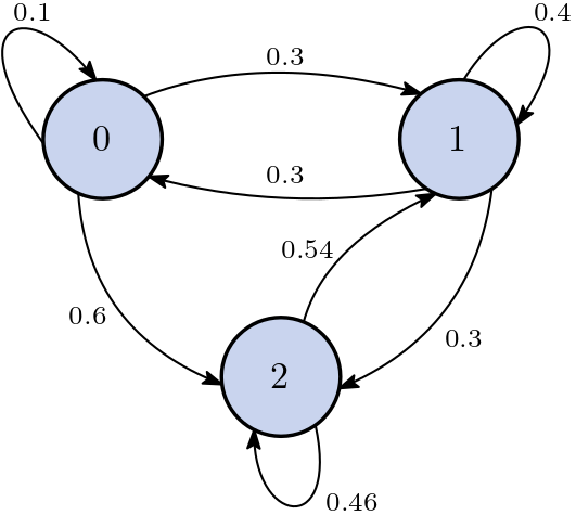
Fig. 78 The Markov chain of this example. Each node represents a degree. Note that there is no transition from degree 2 to degree 0 since its probability is 0.#
A More Complex Example#
Instead of only using the pitch or degree of a scale as elements of the alphabet, we could use complete events played by a Pbind. Furthermore, often you have a lot of transitions that are not possible. Therefore, instead of using a dense matrix, we can use a different data structure that requires less memory. The following is just one of many different possibilities.
Let’s use a list where each entry represents a node.
The node number is equal to the index of the entry.
It should contain the event and the information about the transitions starting at this node.
We model the list by an array which contains an environment.
Here I use the combination of \midinote and \dur as an event.
\nodes is the list of reachable nodes (numbers) and \prob the respective probabilities.
Since I am lazy to compute probabilities, I use normalized weights.
(
~nodes = [
    (\midinote: 60, \dur: 1, \nodes: [1], \probs: [2].normalizeSum),
    (\midinote: 62, \dur: 0.5, \nodes: [0, 2], \probs: [1, 1].normalizeSum),
    (\midinote: 63, \dur: 1, \nodes: [0, 3], \probs: [1, 1].normalizeSum),
    (\midinote: 65, \dur: 0.5, \nodes: [0, 3, 4], \probs: [1, 4, 1].normalizeSum),
    (\midinote: 67, \dur: 1, \nodes: [5], \probs: [1].normalizeSum),
    (\midinote: 70, \dur: 1.5, \nodes: [4, 6], \probs: [1, 2].normalizeSum),
    (\midinote: 69, \dur: 1, \nodes: [4, 7], \probs: [1, 2].normalizeSum),
    (\midinote: 72, \dur: 0.5, \nodes: [4, 7, 0], \probs: [1, 4, 2].normalizeSum),
];
)
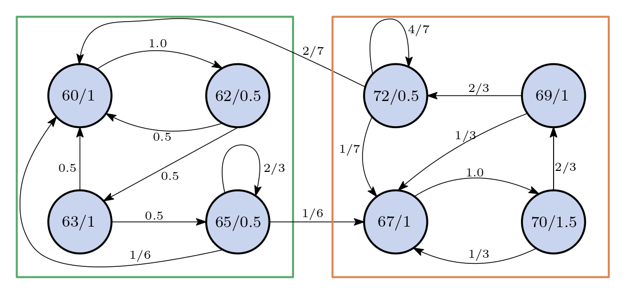
Fig. 79 The Markov chain of this example. Each node represents a degree and duration. There is a low probability that the transition from the green box to the orange box happens.#
Let’s use some custom SynthDef that produces harmonic tones:
(
SynthDef(\saw_approx, {
    var sig, n=20, harmonics;

    harmonics = Array.geom(n, 1, -1) * Array.series(n, 1, 1);

    sig = harmonics.collect({ arg k;
        var env = EnvGen.ar(Env.perc(
            attackTime: \attk.kr(0.01) * Rand(0.8,1.2),
            releaseTime: \rel.kr(5.0) * Rand(0.9,1.1),
            curve: \curve.kr(-4))
        );

        var vibrato = 1 + LFNoise1.ar(\detuneFreq.kr(5)!2).bipolar(\detune.kr(0.015));
        var harmonicFreq = \freq.kr(220) * vibrato * abs(k);
        (1/pi) * SinOsc.ar(harmonicFreq) / k * env.pow(1+((abs(k)-1)/3));
    }).sum;

    sig = LPF.ar(sig, 1500);
    sig = sig * \amp.kr(0.5);
    DetectSilence.ar(sig, doneAction: Done.freeSelf);
    Out.ar(0, sig);
}).add;
)
And let’s use a task running on a clock instead of relying on pattern.
The block is a special function that breaks from the loop.
It calls the receiver with an argument which is a function that returns from the method block.
To exit the loop, one can call .value() or just .() on the function passed in.
One can pass a value to this function and that value will be returned from the block method.
(
var node_index = 0;
var t = TempoClock(2.0);
{
    100.do {
        var node = ~nodes[node_index];
        var dur = node[\dur];
        var freq = node[\midinote].midicps;
        var prob = 1.0.rand;
        var acc = 0;

        node_index = block { |break|
            node[\probs].size.do {|i|
                if((prob < acc), {
                    break.(node[\nodes][i]);
                }, {
                    acc = acc + node[\probs][i];
                });
            }
        };

        Synth(\saw_approx, [
            \rel: dur.linlin(0.5, 1.5, 0.1, 1.0),
            \freq: freq,
            \amp: node[\midinote].linexp(60, 72, 0.8, 0.4)]);
        dur.wait;
    }
}.fork(t)
)
We can definitely hear some pattern of repetition. In both of our examples, we defined the transition probabilities and the nodes by hand. However, it is also possible to analyse a corpus and “learn” the structure to imitate a style.
Higher-order Markov Chains#
To enhance a Markov chain with memory, one calculates the probability of an ensuing event by considering the last \(n\) events instead of solely the most recent one. Such an enriched chain is termed a Markov chain with memory or an \(n^{th}\)-order Markov chain. Despite being time-homogeneous, the potential transitions can proliferate rapidly. Specifically, an \(n^{th}\)-order time-homogeneous Markov chain may necessitate up to
transitions in the most extreme scenario, where \(m\) represents the total number of states.
Crafting an \(n^{th}\)-order chain manually becomes exceedingly intricate when \(n\) exceeds 2. Fortunately, with today’s computational resources, learning higher-order Markov chains from existing data sets has become relatively straightforward. However, transitioning to higher-order chains doesn’t guarantee enhanced or more captivating outcomes. As the order increases, the model tends to fit more closely to the specific data set, a phenomenon known as overfitting. This condition entails nearly perfect memorization of the data set, which paradoxically diminishes the model’s capacity to generate novel and original outputs.
Learning the Chain#
Instead of defining the chain by hand, one can use a corpus of pieces and extract the transition and its probability from it. Let say we have the following piece defined by pairs of midi note and duration.
(
~notes = [
    [74, 0.5],
    [67, 0.25], [69, 0.25], [71, 0.25], [72, 0.25],
    [74, 0.5], [67, 0.5], [67, 0.5],
    [76, 0.5],
    [72, 0.25], [74, 0.25], [76, 0.25], [78, 0.25],
    [79, 0.5], [67, 0.5], [67, 0.5],
    [72, 0.5],
    [74, 0.25], [72, 0.25], [71, 0.25], [69, 0.25],
    [71, 0.5],
    [72, 0.25], [71, 0.25], [69, 0.25], [67, 0.25],

    [66, 0.5],
    [67, 0.25], [69, 0.25], [71, 0.25], [67, 0.25],
    [71, 0.5],[69, 1],

    [74, 0.5],
    [67, 0.25], [69, 0.25], [71, 0.25], [72, 0.25],
    [74, 0.5], [67, 0.5], [67, 0.5],
    [76, 0.5],
    [72, 0.25], [74, 0.25], [76, 0.25], [78, 0.25],
    [79, 0.5], [67, 0.5], [67, 0.5],
    [72, 0.5],
    [74, 0.25], [72, 0.25], [71, 0.25], [69, 0.25],
    [71, 0.5],
    [72, 0.25], [71, 0.25], [69, 0.25], [67, 0.25],

    [69, 0.5],
    [71, 0.25], [69, 0.25], [67, 0.25], [66, 0.25],
    [67, 1.5]
]
)
{
~notes.do ({ |pair|
    Synth(\saw_approx, [freq: pair[0].midicps, rel: 1.1]);
    pair[1].wait;
});
}.fork;
TODO
Summary#
Markov chains present a pivotal probabilistic framework for devising models capable of generating music. These models typically employ time-homogeneous, discrete Markov chains, characterized by either being memoryless or possessing minimal memory. Utilizing such chains enables the manipulation of various aspects of a musical piece, where it is advantageous to govern more abstract, high-level elements like transitions between themes. This approach can mitigate randomness and confer a more structured flow to the composition.
For instance, if a chain is tasked with controlling pitch and permits a broad range of probable transitions, the output can rapidly devolve into cacophony. Such compositions risk becoming overwhelmed by noise, ultimately lacking coherent structure and musicality.