Discrete Fourier Transform#
Up to this point, we considered continuous signals \(y(t)\). In section Fourier Series, we started with continuous periodic functions. We generalized this concept to continuous aperiodic functions in section Fourier Transform. That’s all fine, but on a computer, we are not dealing with continuous functions. On a computer, audio is digitalized. That is, we are dealing with discrete signals.
Definitions#
To deal with a periodic and discrete signal, we switch from the Fourier transform to the discrete Fourier transform. If we want to handle a non-periodic and discrete signal, we apply the discrete-time Fourier transform (DTFT) instead. Because of their similarity, one can easily confuse DFT with the DTFT thus I include this section on Difference between DFT and DTFT at the bottom, but for audio signals, the DTFT is not that relevant.
Discrete Fourier Series (DFS)
The discrete Fourier series \(y: \mathbb{Z} \rightarrow \mathbb{C}\) in exponential form of a periodic and discrete function \(y[n]\) is defined by
which are harmonics of a fundamental frequency \(1/N\), for some positive integer \(N\) (the period of the signal).
This looks very similar to the Fourier series except that \(e^{ikn\frac{2\pi}{N}}\) is a discrete instead of a continuous function. Instead of a sum of continuous functions, the discrete Fourier Series is a sum of discrete functions. Furthermore, there are only \(N\) distinct coefficients \(c^*[0], \ldots, c^*[N-1]\). \(y[n]\) is periodic and so is \(c^*[k]\).
Discrete Fourier Transform (DFT)
The discrete Fourier transform (DFT) transforms a sequence of \(N\) complex numbers \(y[0], \ldots, y[N-1]\) into another sequence of complex numbers \(c[0], \ldots, c[N-1]\), such that
where \(c[k]\) for \(k = 0, \ldots, N-1\) are the coefficients of the discrete Fourier series.
The technique assumes that the samples are equally spaced. The DFT basically uses \(N\) probing functions defined by the phasors \(\hat{1}_{-2 \pi k / N}, k = 0, \ldots, N-1\) to analyse the discrete signal \(y\) for frequencies
times the sample frequency \(f_s\). It produces \(N\) frequency bins and each bin corresponds to a frequency step of
and it covers frequencies in \([0,f_s)\) (or equivalently \([-f_s/2, f_s/2)\) if centered). So the coverage is independent of \(N\)! So \(N\) does not change the maximum frequency you can see—only the resolution between bins.
Example
If \(f_s = 1000\) Hz then \(N=100\) leads to \(\Delta f = 10\) Hz (per bin) in the range \(f_s/N\) to \(f_s\). If \(N=1000\), the resolution increases (not the range), that is, \(\Delta f = 1\) Hz (per bin).
However, due to the Nyquist–Shannon sampling theorem we can only rely on the first half of coefficients, i.e.,
Also, note that the DFT does only probe for frequencies that are an integer multiple of the
It basically assumes that this is the fundamental frequency of the signal. \(N\) samples at a sample rate \(f_s\), span a time window
Therefore, increasing \(N\) (with fixed \(f_s\)) means that we are analyzing a longer time window of the signal. A longer observation leads to better frequency resolution, but poorer time localization (this is the time-frequency tradeoff).
The DFT also implicitly assumes that the \(N\) samples form one period of a period signal and if the signal is not periodic with period \(N\), spectral leakage occurs. So \(N\) also determines the “artificial” period the DFT wraps the signal around.
Therefore, we expect limitations when dealing with inharmonic content because any content within the signal which is not part of some harmonic will be approximated by those harmonics and since we only compute a finite number of coefficients, this approximation is imperfect.
Similar to the Fourier transform there is an inverse transformation.
Inverse Discrete Fourier Transform (IDFT)
The inverse discrete Fourier transform IDFT transforms a sequence of \(N\) complex numbers \(c[0], \ldots, c[N-1]\) into another sequence of complex numbers \(y[0], \ldots, y[N-1]\), such that
where \(c[k]\) for \(k = 0, \ldots, N-1\) are the coefficients of the discrete Fourier transform.
Note that the inverse discrete Fourier transform IDFT is a specific example of a discrete Fourier series.
Example (Perfection)#
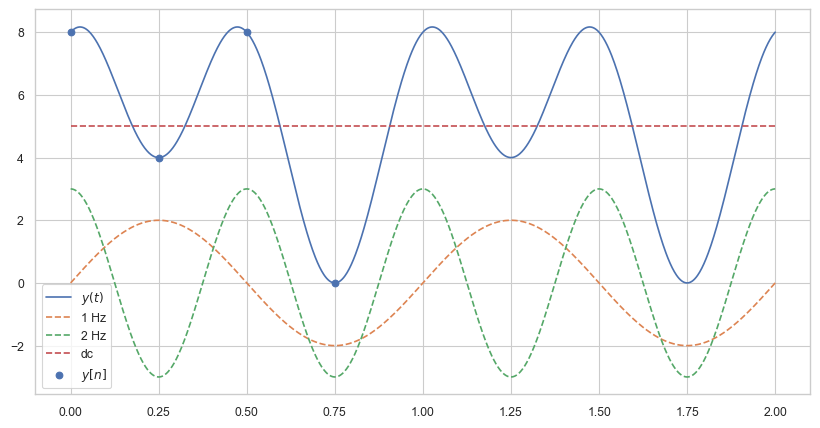
Suppose the following signal is given
The frequency of the fundamental of the signal is 1 Hz and it consists of one additional harmonic. So let us choose a sample rate \(f_s = 4\) Hz that is double the frequency of the highest frequency of the signal. If use \(N=4\), that is, 4 samples \(\Delta f = 1\) Hz and the DFT assumes that \(f_s/N = 1\) is the fundamental. Furthermore, we capture one period we need to sample within \([0;1)\) and all frequencies occuring in the signal. Everything works out.
The values of the discrete samples are given by:
We get \(y[0] = 8\), \(y[1] = 4\), \(y[2] = 8\), \(y[3] = 0\).
Let us implement the DFT and IDFT using sclang.
The following code is inefficient but suffice for our purposes.
DFT#
(
~dft = {arg y, k;
    var m = y.size, result = 0;
    for(0, m-1, {
        arg n;
        result = result + (y[n] * exp(Complex(0,-1) * 2 * pi / m * n * k));
    });
    result;
};
)
y = [8, 4, 8, 0];
c = Array.fill(y.size, {arg i; i}).collect({arg i; ~dft.(y, i)});

/* [
Complex( 20.0, 0.0 ),
Complex( 0.0, -4.0 ),
Complex( 12.0, 1.4695761589768e-15 ),
Complex( -8.8817841970013e-16, 4.0 ) ]
*/
c_k contains the values of our coefficients, i.e. \(c[k]\) for \(k = 0, 1, 2, 3\) Hz, i.e.,
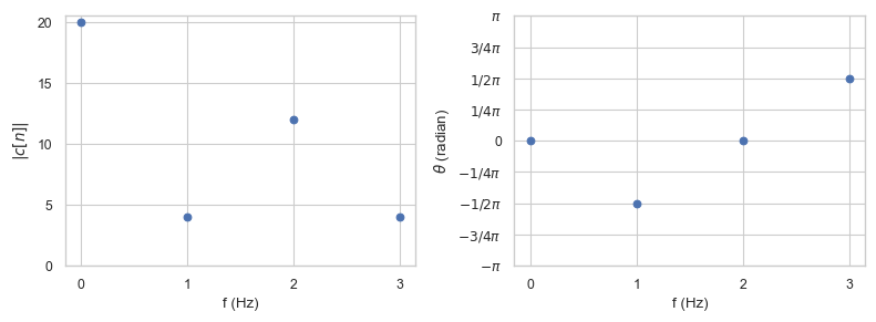
Since we have 4 samples, i.e., \(N=4\), we have to divide by 4 to compute the respective amplitudes. Since \(y(t)\) is a real-valued function we already know that
and the amplitude is given by
otherwise it is
The phase is given by the arctan2
Furthermore, because of Nyquist–Shannon sampling theorem, we can not compute the amplitude (and phase) of frequencies greater than 2 Hz. In general, all \(c[n]\) with \(n > \frac{N}{2}\) are invalid because of aliasing. Therefore, \(c[3] = 4i\) is ‘’incorrect’’. We can not distinguish the sinusoid of frequency \(1\) from the sinusoid of frequency \(3 = 1 + f_s\). Therefore,
In summary, we get
Furthermore, we can perfectly reconstruct the original continuous harmonic signal \(y(t)\)!
Now you might wonder what happened to the complex number \(c[1] = -4i\)? Remember, multiplying by \(i\) equates to a counterclockwise rotation by 90 degrees. The ‘’cosine-part’’ of the complex number represents the real part. Therefore, the phase of the cosine with the fundamental frequency is shifted by \(-\pi/2\). Which is true for \(y(t)\).
IDFT#
Let’s now apply the IDFT:
(
~idft = {arg y, k;
    var m = y.size, result = 0;
    for(0, m-1, {
        arg n;
        result = result + (y[n] * exp(Complex(0,1) * 2 * pi / m * n * k));
    });
    result / m;
};
)
~iy = Array.fill(c.size, {arg i; i}).collect({arg i; ~idft.(c, i)});

/* [
Complex( 8.0, -6.6613381477509e-16 ),
Complex( 4.0, -2.2884754904439e-17 ),
Complex( 8.0, 6.6613381477509e-16 ),
Complex( 7.7715611723761e-16, 1.2475315540518e-15 ) ]
 */
If we neglect the small numerical errors, we get the correct function values \(y[n]\) for \(n = 0, 1, 2, 3\) back again. The imaginary part of the complex numbers is approximately zero because \(y(t)\) is a real-valued function.
Example (Limitation)#
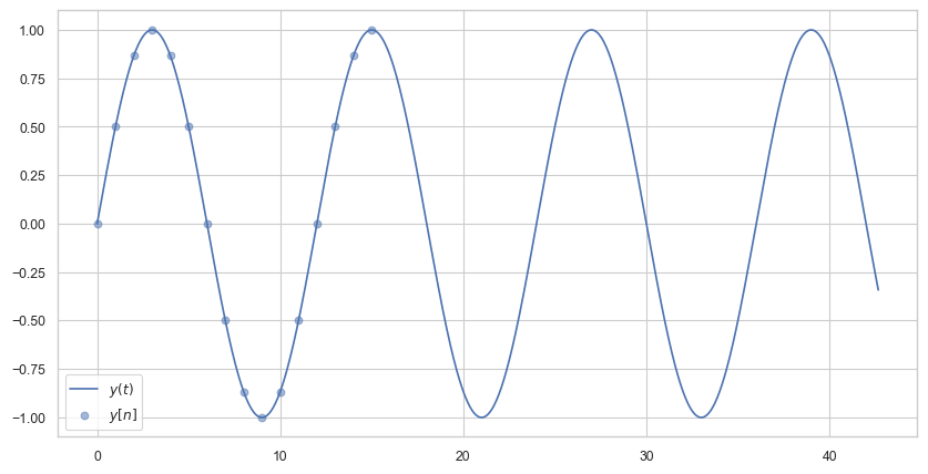
Let us suppose we have the following signal consisting of only one frequency:
Let us assume the analysis period of the DFT is only 16 seconds and the sample frequency \(f_s\) is \(1\) Hertz. Thus \(N = 16\) and \(f_s = 1\) and \(T = N/f_s = 16\) seconds (which is larger than the period of the signal which is 12 seconds).
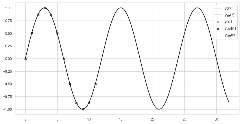
The DFT assumes the fundamental frequency is \(f_s/N = 1/16\) but the frequency of the signal is \(1/12\) which is not a multiple of \(1/16\)! Even though we sample more than one complete period of \(y(t)\) and our sample frequency is much faster than double the frequency of the function, computing the DFT will introduce errors because we introduce a discontinuity because the DFT assumes that after 16 seconds everything repeats, when in fact after 12 seconds it repeats.
The following plot shows the actual signal \(y(t)\) and the discontinuous signal \(y_{\text{dft}}(t)\) ‘seen / assumed’ by the DFT operation. Computing the IDFT gives us the correct sample points, i.e., \(y[n] \equiv y_\text{idft}[n]\) holds, but the reconstructed signal \(y_\text{idft}(t)\) is incorrect.
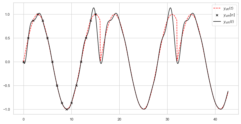
Computing the IDFT gives us the correct values for our samples but if we look at the frequency and phase spectrum we can observe many different frequencies that are present:
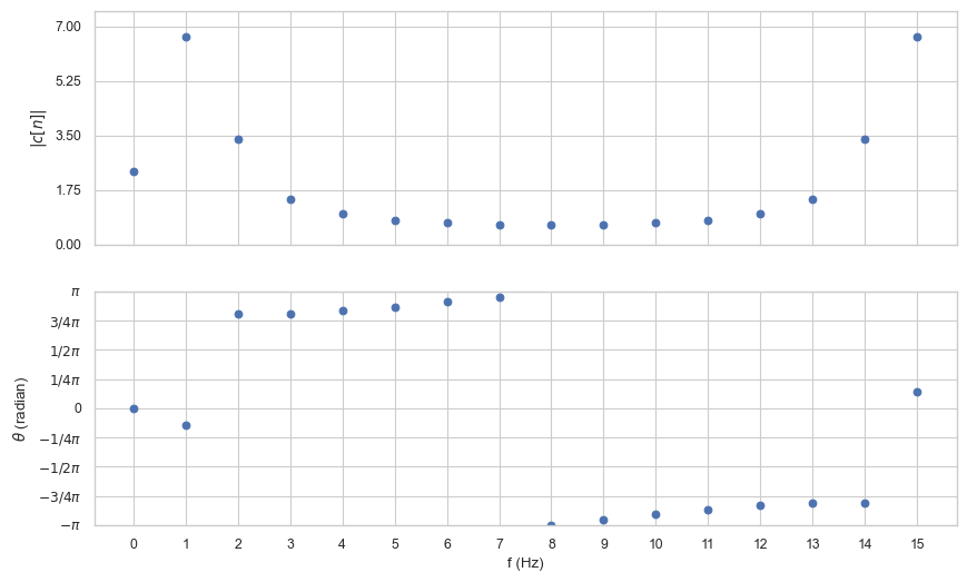
There are actually two problems here:
Picket fence effect: We are trying to represent a frequency \((3/4 \cdot 1/16)\) that is not an integer multiple of the fundamental analysis frequency \(f_N = 1/16\), so the results do not fit appropriately as harmonics of \(f_N\). We cannot view the underlying continuous spectrum because the DFT limits us to integer multiples of the fundamental analysis frequency \(f_N\). This is analogous to observing a row of evenly spaced trees through a picket fence.
Leakage: Discontinuities at the edge of the analysis window spray noise throughout the rest of the spectrum. This phenomenon is called leakage because the energy that should be in one spectral harmonic spreads away (leaks) into adjacent harmonics.
To reduce the picket fence effect, we can increase the spectral frequency resolution by artificially increasing the number of samples, e.g., by padding them with zeros. The leakage problem is more serious. The best we can do is devise a workaround. We create a function exactly as long as the analysis window gradually fades in and fades out at the edges. If we multiply the signal to be analyzed by this function (which is called windowing), we decrease the effect of any discontinuities at the edges of the analysis window because the discontinuities are heavily attenuated at the analysis window edges. This helps to reduce the impact, but there is no free lunch because any alternation of the input signal will have some effect on the resulting spectrum.
The problem can be fixed if we choose \(N=12\). The following plot shows that \(y_{idft}(t)\) is a perfect reconstruction of \(y(t)\).
Fast Fourier Transform#
The fast Fourier transform (FFT) is an algorithm that computes the discrete Fourier transform (DFT) of a sequence, or its inverse. Fourier analysis converts a signal from its original domain (often time or space) to a representation in the frequency domain and vice versa.
The FFT is an efficient way to compute the DFT. It is a divide-and-conquer algorithm that recursively breaks down a DFT of any composite size (a power of 2) into many smaller DFTs. This significantly reduces the computational complexity from quadratic \(\mathcal{O}(n^2)\) to almost linear \(\mathcal{O}(n \log(n))\), which makes it much faster for large sequences.
Let me give you a simplified version of how the Cooley-Tukey radix-2 decimation in time (DIT) FFT [CT65] works. It is one of the most commonly used FFT algorithms.
The algorithm first divides the discrete input signal into two parts: one for even-indexed points and one for odd-indexed points. It computes the DFTs of these two parts recursively. Because the index difference for the odd and even parts is twice as big, half as many points are needed for each DFT, which reduces the computation. The results of the two smaller DFTs are combined into the DFT of the whole signal using a formula called the butterfly operation. The process is repeated until all DFTs are computed.
For more details I refer to the original publication.
Short-Time Fourier Transform#
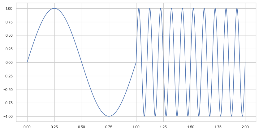
The Fourier transform yields frequency information that is averaged over the entire time domain. Therefore, the information when these frequencies occur is hidden in the transform. For instance, if we have the following signal, and we take the transform, there is no way to tell that the signal’s frequency changed at a certain point in time (here it would be after 1 second).
To recover the hidden time information, Dennis Gabor introduced in 1946, the short-time Fourier transform (STFT). Instead of considering the entire signal, the main idea of the STFT is to consider only a small section of the signal. To this end, one fixes a so-called window function, which is a function that is nonzero for only a short period of time (defining the considered section). The original signal is then multiplied with that window function to get a windowed signal. Then we take the Fourier transform of that windowed signal!
To obtain frequency information at different time instances, one shifts the window function across time and computes a Fourier transform for each of the resulting windowed signals. Each chunk is Fourier transformed, and the complex result is added to a matrix, which records magnitude and phase for each point in time and frequency. This can be expressed as:
where the discrete signal \(y\) is multiplied by the window \(w\). This equation is equal to our definition of the discrete Fourier transform but with the added multiplication of the window \(w\). \(\mathbf{C}\) is no longer a vector but a matrix.
Similar to the measurement processes in quantum physics, there’s an important and rather conspicuous trade-off: it is impossible to measure all frequencies at all times. If we aim for precise timing, we must choose a small windowsize, consequently losing precision in the measured frequencies, meaning we lose low-frequency information.
Conversely, if the windowsize is large, we sacrifice precision in time.
Often one defines a so called hop distance or hop which indicates how far two consecutive windows are apart.
Usually windows overlap.
Furthermore, one can use different window functions (wintype).
SuperCollider supports rectangular -1 windowing (simple but typically not recommended), sine 0 (default) windowing (typically recommended for phase-vocoder work), or Hann windowing 1 (typically recommended for analysis work).
The Hann window looks like a Gaussian bell.
Compared to the sine window, it has an exponential increase and decay, i.e., looks slimmer.
Since we slice over the signal, we get a series of discrete Fourier transforms, one for each timestep. Let us compute the STFT of the following audio signal.
I use a windowsize of 2048 samples and a hop length of 512.
Furthermore, I use the Hann window.
To convert the hop length and windowsize to units of seconds we have to divide it by the sample rate.
shape of matrix C is (1025, 5163)
This STFT has 1025 frequency bins and 9813 frames/windows in time.
Spectrogram#
In music processing, we often only care about the spectral magnitude and not the phase content. The spectrogram shows the intensity of frequencies over time. A spectrogram is simply the squared magnitude of the STFT:
The human perception of sound intensity is logarithmic in nature. Therefore, we are often interested in the log amplitude:
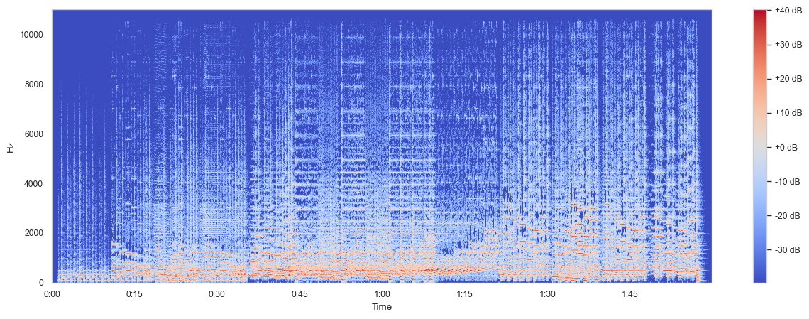
Fig. 22 Spectrogram of the Nutcracker suite.#
Mel-spectrogram#
The Mel frequency cepstral coefficients (MFCCs) are a compact representation of the frequency spectrum. It reduces the full spectrum to the most important aspects.
MFCCs are used for speech, speaker or sound effect recognition or to analyse music to assign metadata to a song or a certain piece of music. In the field of machine learning, they offer a nice representation of a sound (especially since MFCCs as well as spectrograms are images thus a convolutional neural network can deal with these representations).
As we know, when we speak or when any sound is produced, different frequencies of sound are created. These frequencies, when combined, form a complex sound wave. The human ear responds more to certain frequencies and less to others. Specifically, we are more sensitive to lower frequencies (like a bass guitar) than higher frequencies (like a flute), especially at low volumes. This is the concept behind the Mel scale, which is a perceptual scale of pitches that approximates the human ear’s response to different frequencies.
The calculation of the MFCC is an elegant method to separate the excitation signal and the impulse response of the filter. After applying the STFT and throwing away the phase information, we take the logarithm of the amplitude spectrum. This step is performed to mimic the human ear’s response more closely since our perception of sound is logarithmic in nature. Next, we smooth the spectrum and emphasize perceptually meaningful frequencies. To achieve this, we pass the result through a set of band-pass filters called Mel-filter bank. Basically, we merge neighbourhoods of frequencies into one bin. This is to mimic the behavior of the human ear (which is more sensitive to certain frequencies). Since the components of the Mel-spectral vectors calculated for each frame are highly correlated, we try to decorrelate the result to get a more meaningful representation. Therefore, we apply a type of Fourier-related transform called the discrete cosine transform to decorrelate the filter bank coefficients and yield a compressed representation of the filter banks, called the Mel frequency cepstral coefficients. Alternatively, one can use the principal component analysis PCA to achieve a similar effect.
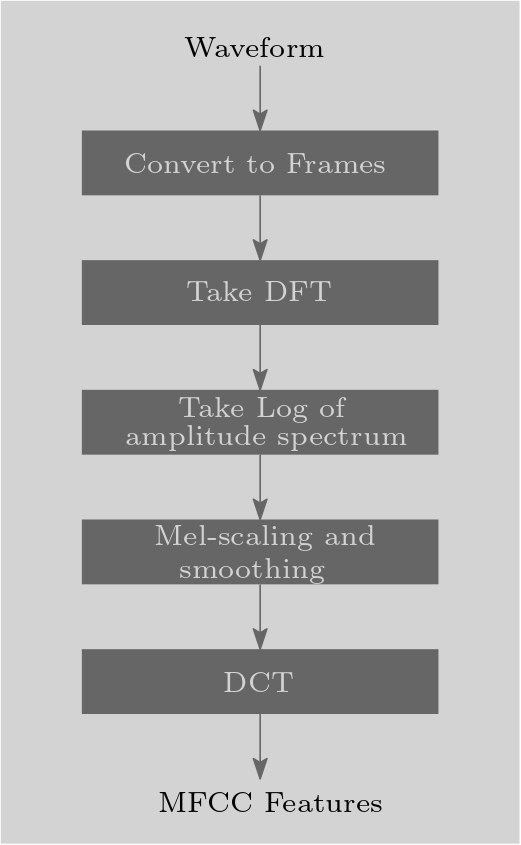
Fig. 23 Process to create MFCC features.#
The Mel filter bank is a collection of overlapping triangular filters that are applied to this spectrum. These filters are not linearly spaced, because they’re designed to mimic the nonlinear frequency resolution of the human auditory system, which is more fine-grained at lower frequencies and coarser at higher frequencies.
The discrete cosine transform (DCT) is used in the MFCC process as a kind of compression step to reduce the dimensionality of the output. It is used to transform the log Mel spectrum (the output of the Mel filter bank) into the time domain. The outputs of each filter in the Mel filter bank are not completely independent of each other; there’s often a lot of correlation because the filters overlap. The DCT is similar to the DFT, but whereas the DFT expresses a signal in terms of complex exponentials (i.e., sinusoids and cosines), the DCT uses only cosines. This is useful because the log Mel spectrum is a real-valued signal, and the symmetry of the cosine function allows for a more compact and efficient representation of such signals than complex exponentials. DCT essentially projects the log Mel filter bank coefficients onto a set of cosine basis functions. These basis functions are much like the “standard patterns” that the filter bank outputs are compared to.
In the following, I use only 13 Mel bands to show the effect.
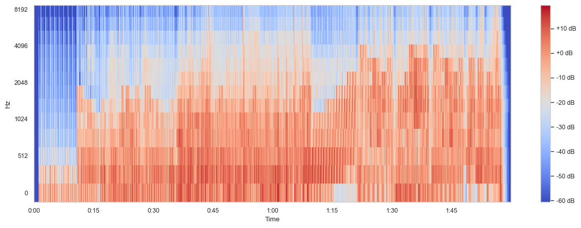
Fig. 24 MFCC of the Nutcracker suite using only 13 bins.#
Difference between DFT and DTFT#
Application: The DTFT is applied to discrete-time signals that are usually obtained from sampling a continuous-time signal. These discrete-time signals are defined over an infinite number of points. The DFT is applied to discrete signals but is particularly useful for signals that are finite in length or are considered to be periodic with a specific period. This makes it ideal for practical computational applications.
Frequency domain representation: The DTFT transforms a discrete-time signal into a continuous function of frequency. The frequency domain representation is continuous and periodic. The DFT transforms a sequence of \(N\) points into another sequence of \(N\) points. Both the input and the output of the DFT are discrete. The frequency domain representation is also discrete and periodic.
Mathematical representation: The DTFT of a signal \(x[n]\) is given by
where \(i\) is the imaginary unit, \(n\) the time index, and \(\omega\) the angular frequency in radians per sample. The DFT of a signal \(x[n]\) is given by
where \(N\) is the number of points in the DFT, \(k\) is the index in the frequency domain, and \(n\) the time index.
Purpose: The DTFT is used to analyze the frequency components of discrete signals that are theoretically infinite in length. The DFT is widely used for signal processing, including filtering, signal analysis, and in the implementation of Fast Fourier Transform (FFT) algorithms for efficient computation.
DTFT is for infinite-length discrete-time signals and results in a continuous frequency spectrum, while DFT is for finite-length signals and results in a discrete frequency spectrum. DTFT’s frequency domain is continuous, whereas DFT’s frequency domain is discrete. DTFT is more theoretical and used for analysis, while DFT is practical and used for computational analysis, especially in digital signal processing. Both of these transforms play crucial roles in signal processing, each suited to different types of problems and analysis.