FFT Processing

Before we start I highly recommand that you read section Discrete Fourier Transform since this section depends on it.

Client Side Computation

Let me first repeat the example from Discrete Fourier Transform using the same sample rate of 4 Hz. First, we define the function

\[y[n] = 5 + 2 \cos(\pi/3 n - \pi/2) + 3 \cos(\pi n)\]

y = { |t| 5 + (2 * cos(2*pi*t-(pi/2))) + (3 * cos(4 * pi * t))}

Then we use the fft call of a Signal which works for real and imaginary signals.

(
var size, real, imag, cosTable, tmp, result;
var sampleRate = 4;
var duration = 2.0;

size = sampleRate * duration;
("size: " ++ size).postln;

tmp = Array.series(size, 0, sampleRate.reciprocal).collect({|t| y.(t)});
real = Signal.fill(size, {|i| tmp[i]});
imag = Signal.newClear(size);
cosTable = Signal.fftCosTable(size);
result = fft(real, imag, cosTable);

("signal: "++real).postln;
("magintutes: "++(result.magnitude/size)).postln;
("phases: "++result.phase).postln;
nil
)

cosTable precomputes a table that speeds up the fft execution. Furthermore, since we have a real-valued signal, our imag signal contains just zeros. The output should show the following:

size: 8.0
signal: Signal[ 8.0, 4.0, 8.0, 0.0, 8.0, 4.0, 8.0, 0.0 ]
magintutes: [ 5.0, 0.0, 1.0, 0.0, 3.0, 0.0, 1.0, 0.0 ]
phases: [ 0.0, 0.0, -1.5707963267949, 0.0, 0.0, 0.0, 1.5707963267949, 0.0 ]

Note that we divide the magnitude by the size of the signal to get the actual amplitudes of the Fourier series y and that

\[1.5707963267949 \approx \frac{\pi}{2}.\]

TODO

Server Side Computation

To compute the DFT and IDFT using the FFT algorithm in SuperCollider (SC), we use the unit generators FFT and IFFT, respectively. And because the fast Fourier transform algorithm is so efficient, we can do it in real time! Therefore, we “work” in frequency space by

1. Transforming the signal into the frequency space using the FFT unit generator

2. Manipulating the coefficients as we desire

3. Transforming the signal back to the time domain using the IFFT unit generator

FFT and IFFT Buffers

FFT and IFFT unit generators require a buffer to store the frequency-domain data. This buffer must have exactly one channel. Multichannel buffers are not supported.

To do FFT processing on a multichannel signal, provide an array of mono buffers, one for each channel. Then, FFT/IFFT will perform multichannel expansion, to process each channel separately.

The following example has no effect on the input ‘in’ since we merely transform the signal and then promptly revert it.

(
{
    var in, out, chain, freq = 200;
    in = SinOsc.ar(freq);

    chain = FFT(
        buffer: LocalBuf(2048), 
        in: in, 
        hop: 0.5, // offset of te next FFT, rnages from > 0 to <= 1.
        wintype: 0, // -1 triangle, 0 sine, 1 Hann
        active: 1, // 1 active, <= 0 inactive
        winsize: 0 // 0 => equal to the buffer
    ); 	

    // here we could manipulate the coefficients
    chain.inspect; 
    out = IFFT(chain); // inverse FFT
    out;
}.play;
)

To process sound SuperCollider has a selection of phase vocoder (PV) unit genertors which are commonly used as in place operators on the FFT data. SuperCollider phase vocoder is a technique used in computer music to manipulate blocks of spectral data before reconversion. The process of buffering, windowing, conversion, overlap-add, etc.

In the following example, we basically filter WhiteNoise by randomly setting most coefficients thus frequencies to zero. Whenever the impulse triggers PV_RandComb and the selection of non-zero frequencies changes. Since the windowsize determines the lowest frequency we can capture, increasing the buffer size will reduce the pitch of the result.

(
{
    var in, chain;
    in = WhiteNoise.ar(0.8);
    chain = FFT(LocalBuf(2048), in);
    chain = PV_RandComb(chain, 0.95, Impulse.kr(0.4));
    IFFT(chain)
}.play;
)

Plotting the spectrogram reveals the effect visually.

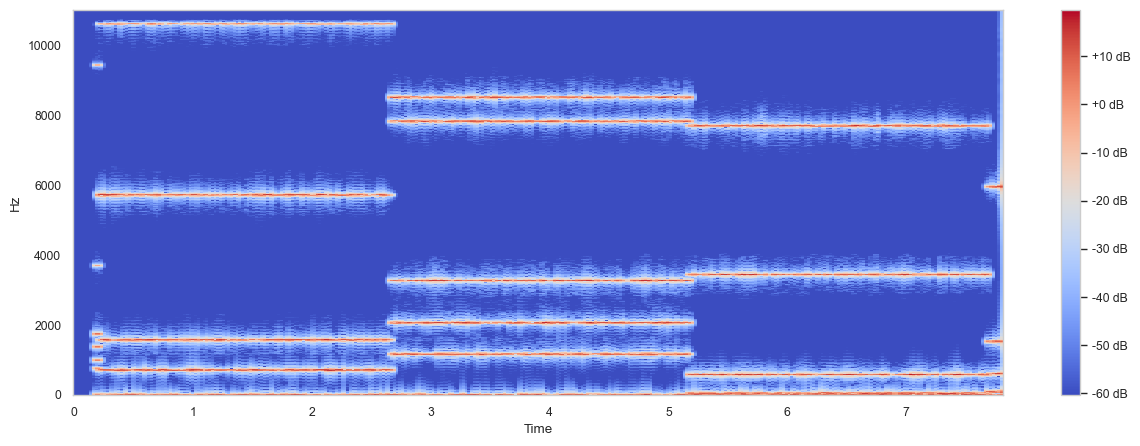
Fig. 68 Spectrogram of the generated signal.

If we want to modify spectral data individually, we can utilize pvcollect. In the following instance, I simulate PV_RandComb by using a random Array named active that contains zeros and ones. Moreover, the operation

index.linexp(b.numFrames, 0, 0.3, 1.0);

reduces the amplitude of high frequencies. To infuse movement, I deploy 2048 low-frequency Pluse unit generators. Since active is smaller than the number frames/windows, i.e. b.numFrames I utilize wrapAt to wrap around. Consequently, a pattern of active frequencies is repeated.

(
{
    var in, chain, b, active, g_amp = 14.0;
    b = LocalBuf(2048);
    active = Array.fill(200, {if(1.0.rand > 0.97, 1, 0)});
    in = PinkNoise.ar();
    chain = FFT(b, in);

    chain = chain.pvcollect(b.numFrames, {|mag, phase, bin, index|
        var factor = index.linexp(b.numFrames, 0, 0.3, 1.0);
        var amp = Pulse.kr(
            rrand(3, 20), 
            rrand(0.1, 0.8)).range(0, 0.9) * factor;
            
        [mag*amp*active.wrapAt(index)*g_amp, phase]
    });

    Pan2.ar(IFFT(chain))
}.play;
)

Again, let us look at the spectrogram:

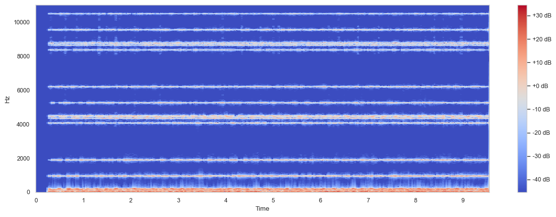
Fig. 69 Spectrogram of the generated signal.

You might notice the repeating frequncy pattern.

TODO

Mel Frequency Cepstral Coefficients

I introduced the mel-spectogram in the section discrete Fourier transform and I recommand reading it before you continue.

In the following example, we use two synth. One creates the audio signal and the other applies a mel-analysis and sends 13 mel-coefficient to a control bus. Every 0.1 second we read from the control bus and store the data in an \(n \times 13\) array.

(
SynthDef(\signal, {
    var sig, n = 25;
    sig = 0;
    n.do {
        arg i;
        var harmonic = SinOsc.ar((i+1)!2 * \freq.kr(440));
        harmonic = harmonic * ((i+1)**2).reciprocal * exprand(1.0, 0.1);
        sig = sig + harmonic;
    };
    sig* 0.5;
    Out.ar(\out.kr(0), sig);
}).add;

SynthDef(\mel, {
    var sig, fft, array;
    sig = In.ar(\in.kr(0));
    fft = FFT(LocalBuf(1024), sig);
    array = MFCC.kr(fft, numcoeff: 13);
    Out.kr(\cout.kr(0), array); // control bus out
    Out.ar(\out.kr(0), Pan2.ar(sig)); // audio bus out
}).add;
)

(
var audio = Bus.control(s, numChannels: 2);
var control = Bus.audio(s, numChannels: 2);
var data = [];

a = Synth(\mel, [in: audio, out: 0, cout: control]);
b = Synth(\signal, [freq: 150, out: audio]);
a.setn(1!13);
	
fork {
    100.do {
        control.getn(13, { |val| { data.add(val); }.defer });
        0.1.wait;
    };
    data.postln;
    a.free;
    b.free;
}.play;
)

Then I plot the data array in Python.

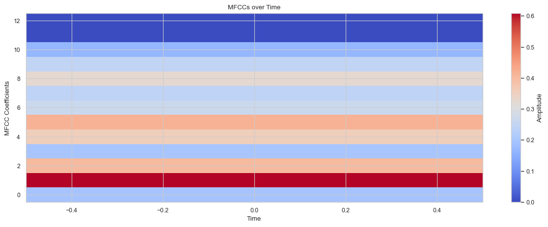
Fig. 70 Mel-spectrogram of the generated signal.

TODO