Frequency Modulation#
Frequency modulation (FM) is the most common encoding technique for public radio transmission (hence FM radio). It uses frequencies that are out of the limits of human hearing. As the name indicates, applying frequency modulation means to modulate the frequency of a signal. In other words, we change the frequency of a signal over time.
Frequency modulation in sound design was accidentally discovered by John Chowning in the mid-60s. He wanted to generate vibrato effects but noticed that when he increased the modulating frequency, a new complex sound appears.
// vibrato example using a low modulation frequency
({
    var sig, freq_car, freq_mod, amp_car, amp_mod;
    freq_car = 300;
    freq_mod = 10;
    amp_car = 0.5;
    amp_mod = freq_car * 0.05;
    sig = amp_car * SinOsc.ar(freq_car + (amp_mod * SinOsc.ar(freq_mod)));
    sig;
}.play;)
Chowning pushed for commercial use but none of the American manufacturers saw the potential of FM. In desperation, Stanford turned to the Japanese manufacturer Yamaha. As a consequence of the success of FM synthesis, the company sold millions of FM synthesizers, organs and home keyboards.
Theory#
Let us start with the very basic equation of a sine wave.
where \(t\) is the time, \(f(t)\) is the frequency and \(A\) the (maximal) amplitude. For frequency modulation, \(f(t)\) is not a constant but a function over time which looks like the following
In summary, we get
which looks very intimidating but don’t worry and just experiment with it!
\(f_\text{car}\) is called carrier frequency, \(f_{\text{mod}}\) modulator frequency and \(A_{\text{car}}\), \(A_{\text{mod}}\) are the respective amplitudes. Those numbers and their relation influence the generated sound fundamentally. We can also use different oscillators and modulate the frequency of the most outer oscillator by multiple modulators!
FM is a very powerful technique to generate a rich spectrum in a very computational efficient way. Above we only use two oscillators but as you will see, we already achieve a quite complex spectrum.
Vibrato & Sirens#
If the frequency of the modulator \(f_{\text{mod}}\) is small, then we achieve a so called vibrato effect. Try the following code snippet!
// another vibrato example
(
Spec.add(\freq_mod, [0.2, 20]);
Spec.add(\freq_car, [50, 1000]);
Spec.add(\amp_mod, [1, 1000]);
Ndef(\fm_low_mod, {
    var mod = SinOsc.ar(\freq_mod.kr(3)) * \amp_mod.kr(5);
    SinOsc.ar(\freq_car.kr(300) + mod) * 0.25 ! 2;
}).play;
)
Ndef(\fm_low_mod).gui;
In this example we use
such that the modulator frequency \(f_{\text{mod}}\) is two magnitudes smaller than the carrier frequency. The effect is a cyclical squeezing and stretching of the carrier waveform. It is astonishing how sensitive human hearing is. We recognize the low frequency within the overall sine wave, i.e., we hear the slowly changing wave shape even if the change is very small. Those small changes result in a vibration similar to the effect of a violinist moving her or his finger on the string in slightly different positions.
Vibrato
There is a unit generator called Vibrato to introduce vibrato after a delay time.
The following sounds similar to the first example above.
// vibrato with 10 Hz wobble,
// starting after 2 second and ramping up over 1 second
// the amplitude is 5 percent of the frequency i.e. 300 * 0.05.
({
    SinOsc.ar(Vibrato.kr(
        freq: 300,
        rate: 10,
        delay: 2,
        depth: 0.05,
        onset: 1)
    ) * 0.25 ! 2;
}.play;
)
If we increase the modulation frequency \(f_{\text{mod}}\) further and further such that it approaches, or even exceeds the carrier frequency \(f_\text{car}\), we get a different effect. At some point, the modulation becomes a form of distortion within the individual cycle of the carrier waveform. To make the distortion more prominent, we have to increase the amplitude of the modulator – a portion of the carrier frequency \(f_{\text{car}}\) is a good starting point.
// fm with a high modulator frequency and amplitude
(
Spec.add(\freq_mod, [1, 2000]);
Spec.add(\freq_car, [1, 1000]);
Ndef(\fm_low_mod, {
    var mod = SinOsc.ar(\freq_mod.kr(800)) * \freq_car.kr(400);
    SinOsc.ar(\freq_car.kr(400) + mod) * 0.5 ! 2;
}).play;
)
Ndef(\fm_low_mod).gui;
In this case, the vibration becomes a wobbling effect or siren-type sound.
Harmonic Relation#
Let us look at this distortion by plotting \(y(t)\) for \(f_{\text{car}} = f_{\text{mod}} = A_{\text{mod}} = \beta = 200\):
(
    ({
    var freq, mod, sig;
    freq = 200;
    mod = SinOsc.ar(freq) * freq;
    sig = SinOsc.ar(freq + mod);
    sig;
}).plot(1/(200));
)
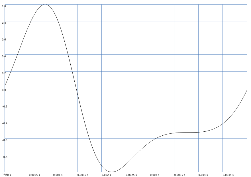
Fig. 65 One cycle of \(y(t)\) for a high frequency modulation frequency.#
If we look at the stethoscope, we observe multiple sidebands, i.e., there are numerous frequencies apart from the fundamental frequency (which is equal to the carrier frequency) present. How many frequencies are present? Well, in theory, an infinite amount! Fortunately, there is a formula for the frequencies \(f_{\text{sb},n^{\pm}}\) of the sidebands
with \(n \in \mathbb{N}\).
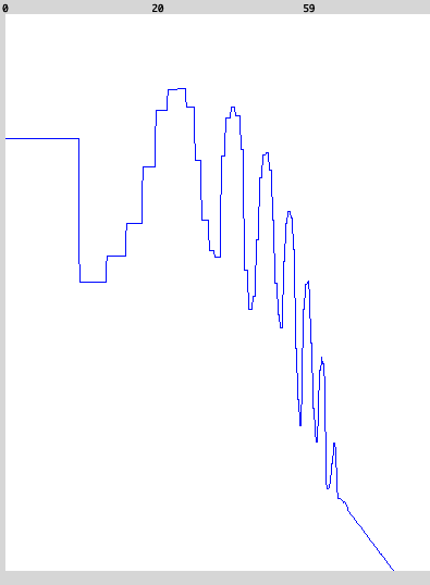
Fig. 66 Snapshot of the stethoscope using a logarithmic frequency scale (\(x\)-axis).#
If we want to keep the same sideband relation for different carrier frequencies, we have to compute the modulation frequency based on the carrier frequency. In other words, we have to correlate these two frequencies.
Sideband Frequencies
A linear relation between \(f_\text{car}\) and \(f_\text{mod}\) keeps the sidebands similar.
Therefore, it is useful to introduce a ratio:
such that
// fm using the ratio to keep the bandwidth realtion the same
// while varying the carrier frequency
(
Spec.add(\ratio, [1/10, 10]);
Spec.add(\freq_car, [1, 1000]);
Ndef(\fm_low_mod, {
    var freq_mod = \freq_car.kr(400) * \ratio.kr(1);
    var mod = SinOsc.ar(freq_mod) * \freq_car.kr(400);
    SinOsc.ar(\freq_car.kr(400) + mod) * 0.5 ! 2;
}).play;
)
Ndef(\fm_low_mod).gui;
Sideband Amplitudes#
The question is now: what about the amplitudes of the sidebands? We already observed what happens if the modulation frequency is low and we increase the modulator amplitude. We achieved a gentle vibrato effect for low amplitudes, but for large amplitudes, this transforms into a siren-type sound.
For high modulation frequencies, we can transfer this phenomenon. The amplitude of the modulator will determine the amplitude of the sidebands. This implies that we can not control the amplitude of each individual sideband. We can only control their amplitudes as a whole!
Also, the modulator’s amplitude is not solely responsible for this effect, but the relationship between it and the modulation frequency \(f_{\text{mod}}\). The so-called modulation index gives us this relationship. It is equal to the ratio of frequency deviation of \(y(t)\) and the modulation frequency \(f_{\text{mod}}\):
We can compute the maximum modulation index \(\beta_{\text{max}}\) by
If we want to have approximately the same harmonic relationship for all keys on the keyboard, we have to change both \(f_{\text{car}}\) and \(f_{\text{mod}}\) accordingly while playing. However, if we also want the same tone, we also have to adapt \(A_{\text{mod}}\) such that \(\beta_{ \text{max} }\) stays approximately constant, that is, we compute \(A_{\text{mod}}\) by
and fix \(\beta_{\text{max}}\) as we desire.
Modulation Index
The modulation index \(\beta_{\text{max}}\), i.e., ratio of the modulation amplitude and the modulator frequency determines approximately the amplitudes of the sidebands as a whole.
Ok, but wait, we still have no formula for the amplitude of each pair of sidebands with frequency \(f_{\text{sb},n^{\pm}}\). This amplitude is given by the Bessel function (of first kind):
The series is a converging series and especially in our case where \(\beta_\text{max}\) is not too large, the values of each term become very small very quick.
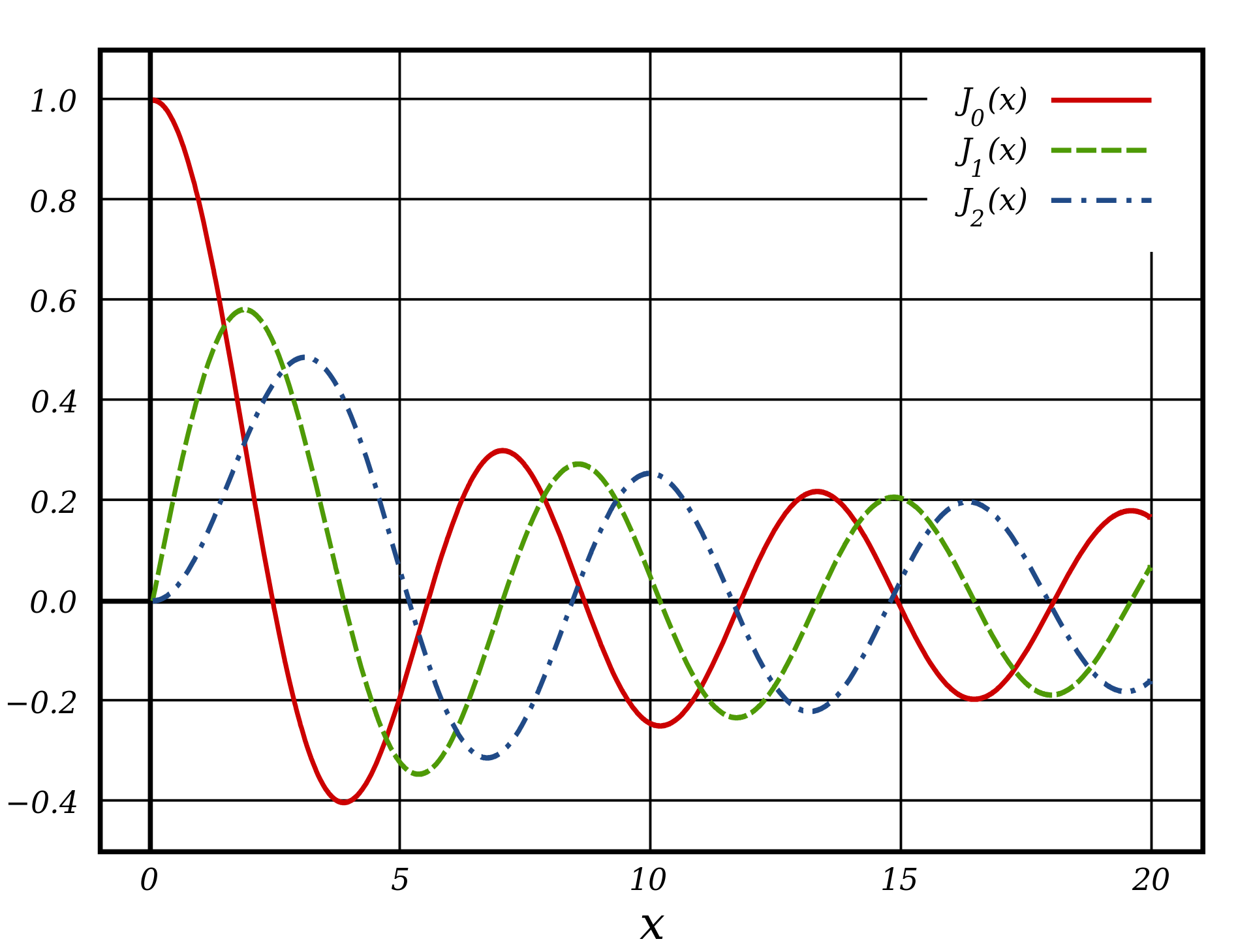
Fig. 67 Plot of Bessel function of the first kind, \(J_n(x)\), for integer orders \(n = 0, 1, 2\). Figure made by Inductiveload - Own work, made with Inkscape, Public Domain, link.#
As we can see, \(A_{ \text{sb},n^{\pm} }\) depend only on \(\beta_\text{max}\) but oscillate for increasing \(\beta_\text{max}\)!
Bandwidth#
We stated that there are an infinite amount of sidebands. In practice, that is not the case. Furthermore, the amplitude of many of these sidebands might be too low to be recognized by our ears. As a rule of thumb, the following formula gives an approximation of the bandwidth of the signal:
Again the modulation index will determine the bandwidth. The larger the index, the larger the bandwidth.
Summary#
Given \(f_\text{car}\), \(r_\text{mod}\), \(\beta_\text{max}\) we compute \(f_\text{mod}\) and \(A_\text{mod}\) by
Example#
The following example is an FM synth heavily inspired by the tutorial given by Alik Rustamoff.
It uses the relations above, but instead of using only one modulator, we use three.
In the code f is \(f_\text{car}\), modFreq1 is \(f_\text{mod}\), \ratio1 is \(r_\text{mod}\) and \modIndex1 represents \(\beta_\text{max}\).
Furthermore, we added some naturalization (distortion and more) to achieve a more gentle result.
(
SynthDef(\fm, {
    var sig, f, car, env;
    var modFreq1, modFreq2, modFreq3;
    var mod1, mod2, mod3;
    var ampmod1, ampmod2, ampmod3;


    // noisy envelope
    env = EnvGen.ar(Env.perc(
        \att.kr(0.015) * Rand(0.8,1.2),
        \rel.kr(4.0) * Rand(0.9, 1.1),
        curve: \curve.kr(-4)
    ),
    doneAction: Done.freeSelf);
    env = env * PinkNoise.ar(1!2).range( 0.1, 1 ).lag(0.01);

    // f = f_car
    f = \freq.kr(220);

    // (11.4a) f_mod = f_car * r^{-1}_mod + distortion
    modFreq1 = f * \ratio1.kr(2).reciprocal + {Rand(-2, 2)}.dup;
    modFreq2 = f * \ratio2.kr(3).reciprocal + {Rand(-2, 2)}.dup;
    modFreq3 = f * \ratio3.kr(4).reciprocal + {Rand(-2, 2)}.dup;

    // (11.4b) A_mod = f_mod + beta_max
    ampmod1 = modFreq1 * \modIndex1.kr(1);
    ampmod2 = modFreq2 * \modIndex2.kr(0.5);
    ampmod3 = modFreq3 * \modIndex3.kr(0.8);

    // (partly 11.2 multiplied with env) A_mod * sin(2pi*f_mod t)
    // effectively reduces the modulation index beta_max over time
    mod1 = SinOsc.ar(modFreq1) * ampmod1 * env;
    mod2 = SinOsc.ar(modFreq2) * ampmod2 * env;
    mod3 = SinOsc.ar(modFreq3) * ampmod3 * env;

    // (11.1 or 11.3) y(t) = A_car * sin(f_car + A_mid * sin(2pi*f_mod t) t)
    car = \amp.kr(0.5) * SinOsc.ar(
        // f_car
        f +
        // changes the effective carrier frequency over time (low frequency) [\pm 5 * 10^{-3} * f_car; 0]
        LFTri.ar(
            freq: env.pow(0.5) * LFNoise1.kr(0.3).range(1,5),
            iphase: Rand(0.0,2pi),
            mul: env.pow(0.2) * f * 0.005) +
        // distortion [-f/8; +f/8] but the noise is smoothen (it imitates a Brownian motion).
        WhiteNoise.ar(f/8!2).lag(0.001) +
        // f_mod
        [mod1,mod2,mod3].sum);

    // add some envelope
    sig = car * env;
    sig = HPF.ar(sig, f);
    sig = LPF.ar(sig, f);
    Out.ar(0, sig);
}).add;
)
Let us play the synth:
(
Pbindef(\melody3,
    \instrument, \fm,
    \dur, Pshuf(2.pow((-4..1)), inf),
    \degree, Pshuf([0, 2, 5, 6, 8, 11], inf),
    \octave, Pdup(Prand([2,3,4], inf), Pseq([3,4,5], inf)),
    \ratio1, Prand([1,2,3,4], inf),
    \ratio2, Prand([3,4,5], inf),
    \amp, 1.0
).play;
)