Physical Modeling#
To achieve a sound synthesis method that authentically replicates the characteristics of real musical instruments, it’s imperative to consider the underlying physics governing these instruments. Physical modeling synthesis relies on mathematical equations derived from the field of acoustics, which, although challenging to construct and control, offer the closest approximation to the genuine sound of instruments, second only to the less expressive method of sampling [Col].
Physical modeling in sound design refers to a technique used to synthesize or replicate sound by simulating the physical properties and behaviors of real-world acoustic and mechanical systems. Instead of using traditional methods like sample playback or subtractive synthesis, physical modeling aims to recreate sounds by mimicking the way sound is generated in the real world.
Sound designers and engineers create mathematical models that describe the physical characteristics of a sound-producing system. This system could be a musical instrument, a room, a vibrating object, or any other sound source. These mathematical models simulate the physical processes that occur when sound is generated. This can include modeling the vibration of strings, the resonance of a cavity, the interaction of air molecules, and more. Physical modeling synthesizers or software allow for real-time interaction with these models. Parameters can be adjusted to control various aspects of the sound, such as pitch, timbre, and dynamics. By accurately modeling the physical properties and behaviors of the source, physical modeling can produce highly realistic and expressive sounds that capture the nuances and subtleties of acoustic instruments and other sound-producing systems.
It is commonly used for creating realistic simulations of acoustic instruments like pianos, guitars, and violins, as well as for synthesizing unique and experimental sounds that may not be achievable with traditional synthesis methods. It’s particularly useful in virtual instrument plugins and digital synthesizers, where it can provide a wide range of sonic possibilities and expressive control over the generated sounds.
One downside of physical modeling is its performance requirements. Solving differential equations is costly. Therefore, easy to use real time models are in many cases still out of reach. There are however an increasing number of successful designs, and certainly bound to be more to come.
According to Collins [Col] there are a number of techniques in physical modeling, including:
modal synthesis: being a study of the exact modes of vibration of acoustic systems: related to analysis + additive synthesis
delay line (waveguide) models: (building physical models out of combinations of simple units like delays and filters, which model the propagation of sound waves in a medium)
mass-spring models: based on dynamical equations; elementary masses and springs can be combined into larger models of strings, membranes, acoustic chambers, instrument bodies…
Collins offers us the following example adapted from [RF95]:
(
var modes,modefreqs,modeamps;
var mu,t,e,s,k,f1,l,c,a,beta,beta2,density;
var decaytimefunc;
var material;

material= \nylon; // \steel

//radius 1 cm
a=0.01;
s=pi*a*a;

//radius of gyration
k=a*0.5;

if (material == \nylon, {
    e=2e+7;
    density=2000;
},{//steel
    e = 2e+11; // 2e+7; //2e+11 steel;
    //density p= 7800 kg m-3
    //linear density kg m = p*S
    density=7800;
});

mu=density*s;
t=100000;
c = (t/mu).sqrt;	//speed of sound on wave
l=1.8;	//0.3
f1= c/(2*l);
beta= (a*a/l)*((pi*e/t).sqrt);
beta2=beta*beta;
modes=10;
modefreqs = Array.fill(modes,{
    arg i;
    var n,fr;
    n=i+1;
    fr=n*f1*(1+beta+beta2+(n*n*pi*pi*beta2*0.125));

    if(fr>21000, {fr=21000}); //no aliasing
    fr
});

decaytimefunc= {arg freq;
    var t1,t2,t3;
    var m,calc,e1dive2;

    m = (a*0.5)*((2*pi*freq/(1.5e-5)).sqrt);
    calc = 2*m*m/((2*(2.sqrt)*m)+1);
    t1 = (density/(2*pi*1.2*freq))*calc;
    e1dive2 = 0.01;
    t2 = e1dive2/(pi*freq);

    t3 = 1.0/(8*mu*l*freq*freq*1);
    1/((1/t1)+(1/t2)+(1/t3))
};

modeamps=Array.fill(modes,{arg i; decaytimefunc.value(modefreqs.at(i))});
modefreqs.postln;
modeamps.postln;

{
    var sig, env;
    env = EnvGen.ar(Env([0,1,1,0],[0,10,0]), doneAction: 2);
    sig = Mix.fill(modes, {
        arg i;
        XLine.ar(1.0, modeamps.at(i), 10.0) * SinOsc.ar(modefreqs.at(i), 0, 1.0/modes)
    });

    sig = env * sig;
    Pan2.ar(sig,0)
}.play;
)
Modeling sound with an exciter and a resonator is a common approach in physical modeling synthesis. This technique is used to simulate the behavior of acoustic instruments, such as stringed instruments like guitars or pianos. Here’s a basic overview of how it works:
Exciter: The exciter is responsible for initiating the vibration in the physical model. In many cases, it represents the initial force applied to the sound source. In stringed instruments, this could be a pluck or a strike on the string.
Resonator: The resonator represents the body or acoustic chamber of the instrument where sound waves resonate and develop their unique timbre. It consists of one or more resonating elements that shape the sound as it evolves over time.
(
{
    var exciter, decay, noise;
    exciter = Impulse.ar(0.01);
    decay = Decay2.ar(exciter, 0.008, 0.04);
    noise = LFNoise2.ar(3000) * decay;
    noise
}.play;
)
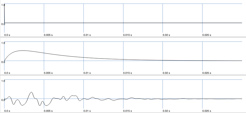
Fig. 71 Plot of the three generated signals. A very simple exciter as an impulse, the decay of the impulse combined with noise representing the resonator.#
Instead of using LFNoise2 we could have also used some other noise generator such as WhiteNoise. If we introduce reverberation, we get a much more pleasant result. First, let us use white noise. Second, let us add a delay line.
(
SynthDef(\delay, {
    var sig, exciter, local;

    local = LocalIn.ar(2);
    exciter = Impulse.ar(0!2);
    sig = WhiteNoise.ar() * exciter;
    sig = sig + local;

    local = DelayN.ar(sig, 0.01,
        delaytime: \delaytime.kr(0.002)) * \beta.kr(0.95);
    LocalOut.ar(local);

    DetectSilence.ar(sig, doneAction: Done.freeSelf);
    Out.ar(0, sig);
}).add;
)

Synth(\delay, [beta: 0.98, delaytime: 0.002]);
Adding filters gives us control over the frequency of the signal. Here I use the default low pass filter.
(
SynthDef(\delay, {
    var sig, exciter, local;

    local = LocalIn.ar(2);
    exciter = Impulse.ar(0!2);
    sig = WhiteNoise.ar() * Decay2.ar(exciter, 0.008, 0.04) * \amp.kr(1.0);
    sig = sig + local;
    sig = LPF.ar(sig, \cutoff.kr(440));

    local = DelayN.ar(sig, 0.01,
        delaytime: 1/\freq.kr(440)) * \beta.kr(0.95);

    LocalOut.ar(local);

    DetectSilence.ar(sig, doneAction: Done.freeSelf);
    Out.ar(0, sig);
}).add;
)

(
Pbind(
    \instrument, \delay,
    \dur, Pseq([0.25, 0.25, 0.5, 0.5, 0.25], inf),
    \cutoff, Pexprand(1000, 6000, length: 30),
    \beta, 0.97,
    \midinote, Pseq([65, 70, 80, 54], inf),
    \amp, 1,
    \pan, (Pkey(\midinote).linlin(54, 80, -0.9, 0.9))
).play;
)
A simplified variant of physical modeling sound synthesis, akin to what we’ve discussed earlier, is known as the Karplus-Strong synthesis. Here, the process commences with a noise source placed within a delay line, its length determined by the desired note’s pitch. Subsequently, the delay line undergoes successive filtering until the sound completely diminishes. This technique yields a periodic sound due to the fixed length of the loop, represented by the delay line.
The previous examples share some resemblance with this approach, as a comb filter essentially functions as a recirculating delay line.
A fundamental limitation of doing it this way is that any feedback (here achieved using a LocalIn and LocalOut pair) acts with a delay of the block size (64 samples by default).
In this context, the filter serves to gradually attenuate the sound over time, while the length of the delay line corresponds to the resulting waveform’s period.
The maximum frequency this system can cope with is SampleRate.ir/ControlDur.ir, which for standard values is 44100/64, about 690 Hz.
So more accurate physical models often have to be built as individual unit generators, not out of unit generators.
Consequently, there is a readymade Karplus-Strong synthesis unit in SuperCollider, that is, the Pluck unit generator:
(
SynthDef(\pluck, {
    var sig, exciter, local;

    sig = Pluck.ar(
        in: WhiteNoise.ar(0.1!2), trig: Impulse.kr(0),
        maxdelaytime: \freq.kr(440).reciprocal,
        delaytime: \freq.kr(440).reciprocal,
        decaytime: 10,
        coef: \coeff.kr(0.3)
    );

    DetectSilence.ar(sig, doneAction: Done.freeSelf);
    Out.ar(0, sig);
}).add;
)

(
Pbind(
    \instrument, \pluck,
    \dur, Pseq([0.25, 0.25, 0.5, 0.5, 0.25], inf),
    \midinote, Pseq([65, 70, 80, 54], inf),
    \amp, 1,
    \coeff, Pwhite(-0.1, 0.1, length: 30),
    \pan, (Pkey(\midinote).linlin(54, 80, -0.9, 0.9))
).play;
)
Some useful filter UGens for modelling instrument bodies and oscillators for sources: