Complex Numbers

The history of mathematics is a rich tapestry of discoveries and inventions. The Greeks, fascinated by geometry, introduced both natural and rational numbers but, intriguingly, neglected to incorporate negative numbers or zero. Their experiences and understanding of the world, their perspectives on points, lines, and shapes – grounded in classical Euclidean geometry—kept these concepts hidden. Negative lengths or areas were unheard of. They also seemed aware that there might be another category of number—the irrational numbers—beyond the rational. Legend has it that a student of Pythagoras stumbled upon this notion, asserting that something other than rational numbers must exist for the existing mathematical theories to hold true. His audacity cost him his life.

As the world evolved, so did mathematical concepts. The advent of sophisticated financial systems, underscored by the principles of credit and debt, gave birth to the concept of negative numbers. After all, the balance between debt and credit necessitated the existence of a counterpart to a positive number in terms of addition.

We rely on natural numbers to solve equations like \(2x = 4\). We require negative numbers for equations like \(2x = -4\), rational numbers for equations such as \(4x = 2\), and real numbers to tackle equations like \(x^2 = 2\). So, how do we approach the solution for

(2)\[x^2 + 2 = 0?\]

We require complex numbers. These numbers extend real numbers by definition, but their definition is not arbitrary. Instead, it has been meticulously crafted so that complex numbers possess all necessary properties to be integrated into all known and accepted theories. To define complex numbers, we introduce a special symbol \(i\) (some prefer to use \(j\)), which is defined as follows imaginary number:

(3)\[i^2 := -1.\]

We can define \(i\) in a self-referential manner and it was Spencer-Brown [SB69] who thought about such paradoxical definitions as generator:

\[i \leftarrow -1/i.\]

Assuming, we initialize \(i\) with one, this generator would generate the following oscillation: \(-1, 1, -1, 1, \ldots \) which is an interesting perspective. However, in general, we just use the static definition above without the need for the involvement of time. Again, complex numbers are invented but they are also discovered because everything works out, i.e., they have all the rich mathematical properties we desire and require. Let us solve Eq. (2):

\[x^2 = -2 = 2 i^2 \iff x = \sqrt{2i^2} = \sqrt{2} \sqrt{i^2} = \sqrt{2}i\]

sclang provides a class called Complex. Objects of that class represent complex numbers. Let us solve Eq. (2) with sclang:

n = Complex(real: -2, imag: 0) // -2
x = sqrt(n)                    // i*sqrt(2)

For complex numbers to be useful, they must be compatible with real numbers. For instance, what does the expression \(i + 3\) represent, where \(i\) is a complex number and \(3\) is a real number?

Complex Numbers

A complex number

(4)\[\begin{equation} z = (a + bi) \in \mathbb{C}, \end{equation}\]

with \(i = \sqrt{-1}\), is the sum of a real number \(a = \textbf{Re}(z) \in \mathbb{R}\) and an imaginary number \(b = \textbf{Im}(z)\).

A complex number \(z\) has two parts: a real real and an imaginary imag part. Note that squaring an imaginary number gives a real number, i.e. \((bi)^2 = -1b^2 = -b^2\). Furthermore, we get \(0 = 0 + 0i\), \(bi = 0 + bi\), \(a = a + 0i\).

Equality, addition, multiplication and negation works as expected. There is however an additional special operation called complex conjugation.

Complex Conjugation

The conjugation \(\overline{z}\) of a complex number \(z = a + bi\) is the negation of its imaginary part, i.e.,

(5)\[\begin{equation} \overline{z} = \overline{a + bi} = \overline{a} + \overline{bi} = a - bi. \end{equation}\]

n = Complex(real: 2, imag: 9)
n.conjugate // Complex(real: 2, imag: -9)
n.conjugate * n // Complex(real: 85, imag: 0)

Multiplying a complex number \(z = a + bi\) by its conjugate gives us a real number:

\[z \cdot \overline{z} = (a + bi) \cdot (a - bi) = a^2 - (bi)^2 = a^2 + b^2.\]

We can use this fact to evaluate the division of two complex numbers \(z_1 = a + bi, z_2 = c + di\):

\[\frac{a + bi}{c + di} = \frac{(a + bi)(c - di)}{(c + di)(c - di)} = \frac{ac-adi+bic+bdi^2}{c^2+d^2} = \frac{(ac+bd) + (bc-ad)i}{c^2+d^2}.\]

For example:

\[\frac{2 + i}{3 + 2i} = \frac{(2 + i)(3-2i)}{(3 + 2i)(3-2i)} = \frac{6 -4i + 3i -2i^2}{3^2 + 2^2} = \frac{8 -i}{13}.\]

Complex(2, 1) / Complex(3, 2)

Complex Plane

We can represent a complex number \(z = a + bi\) by a point \((a, b)\) in the Cartesian plane, which we then call complex plane or \(z\)-plane.

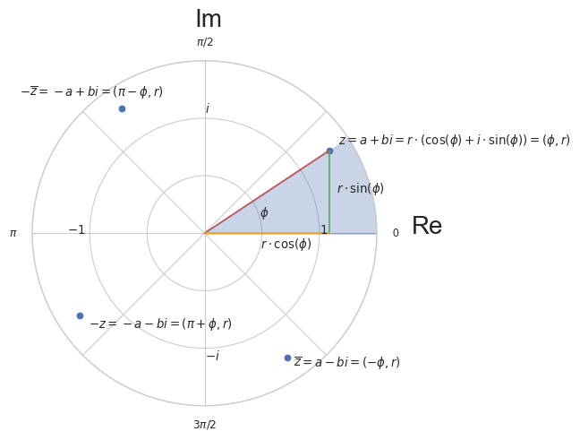
This gives us another representation using the angle \(\phi\) and the magnitude \(r\) of the vector \((a, b)\). We have

(6)\[\begin{equation} \begin{split} a &= r \cdot \cos(\phi)\\ bi &= r \cdot i\sin(\phi) \end{split} \end{equation}\]

thus

(7)\[\begin{equation} \begin{split} z &= a + bi\\ &= (r \cdot \cos(\phi)) + (r \cdot i \sin(\phi))\\ &= r \cdot (\cos(\phi) + i \sin(\phi)). \end{split} \end{equation}\]

We write \(z = (r, \phi)\), \(z = a + bi\), \(z = r \cdot (\cos(\phi) + i \sin(\phi))\) interchangeable. Given \(a\) and \(b\), we can compute \(r\) by

(8)\[\begin{equation} r^2 = a^2 + b^2 = z \cdot \overline{z} \end{equation}\]

and \(\phi\) using

(9)\[\begin{equation} \phi = \cos^{-1}(a/r). \end{equation}\]

Furthermore we can compute \(\phi\) if only \(a\) and \(b\) are given using the arctan2 function

(10)\[\begin{equation} \phi = \text{arctan2}(b, a). \end{equation}\]

(
var theta = 0.25*pi;
var z = Complex(cos(theta), sin(theta));
theta.postln;      // 0.78539816339745
z.postln;          // Complex( 0.70710678118655, 0.70710678118655 )
z.asPolar.postln;  // Polar( 1.0, 0.78539816339745 )
)

What happens geometrically if we multiply two complex numbers? If one of the numbers is a real number, we just scale the magnitude.

Let \(z_1 = r_1 \cdot (\cos(\alpha) + i \sin(\alpha))\) and \(z_2 = r_2 \cdot (\cos(\beta) + i \sin(\beta))\) then

(11)\[\begin{split}\begin{split} z_1 \cdot z_2 &= r_1 \cdot (\cos(\alpha) + i \sin(\alpha)) \cdot r_2 \cdot (\cos(\beta) + i \sin(\beta))\\ &= r_1r_2 \cdot (\cos(\alpha)\cos(\beta) + i\cos(\alpha)\sin(\beta) + i \sin(\alpha)\cos(\beta) + i^2 \sin(\alpha)\sin(\beta))\\ &= r_1r_2 \cdot [(\cos(\alpha)\cos(\beta) - \sin(\alpha)\sin(\beta)) + i (\cos(\alpha)\sin(\beta)+\sin(\alpha)\cos(\beta))] \\ &= r_1r_2 \cdot [\cos(\alpha+\beta) + i \sin(\alpha+\beta)]. \end{split}\end{split}\]

The last step requires the trigonometry identities

\[\begin{equation*} \cos(\alpha)\cos(\beta) - \sin(\alpha)\sin(\beta) = \cos(\alpha + \beta) \end{equation*}\]

and

\[\begin{equation*} \cos(\alpha)\sin(\beta)+\sin(\alpha)\cos(\beta) = \sin(\alpha + \beta). \end{equation*}\]

Eq. (11) gives us some insights. The product of two complex numbers equates to scaling and rotating by magnitude and angle of the second number respectively.

Product of Complex Numbers

The product of two complex numbers is the product of their magnitudes and the sum of their angles.

Since \(i = 1 \cdot (a \cos(90) + i\sin(90))\) holds, multiplying by \(i\) equates to a counterclock rotation by 90 degrees. Since \(-i = 1 \cdot (a \cos(90) - i\sin(90)) = 1 \cdot (a \cos(90) + i\sin(-90))\), dividing by \(i\) equates to multiplying by \(-i\) thus

\[\frac{1}{i} = -i\]

and

\[\frac{1}{i} \cdot \frac{1}{i} = (-i)(-i) = -1.\]

From the rule of products of complex numbers de Moivre’s Theorem follows.

De Moivre’s Theorem

Let \(z = r \cdot (\cos(\phi) + i \sin(\phi))\) be a complex number, then

(12)\[\begin{equation} z^n = r^n (\cos(n\phi) + i \sin(n\phi)) \end{equation}\]

holds.

Euler’s Formula

Euler’s formula or Euler’s equation is one of the most beautiful relationships one can think of. It connects Euler’s number \(e\), \(0\), \(1\) and \(\pi\). To arrive at the formula we first have to do some work.

Taylor Sries

Let \(y(t)\) be a real or comlex-valued function that is infinitely differentiable at a real or complex number \(z,\) then

(13)\[\begin{equation} \begin{split} T_{y(z)}(t) &= y(z) + \frac{y'(z)}{1!}(t-z) + \frac{y''(z)}{2!}(t-z)^2 + \frac{y'''(z)}{3!}(t-z) + \ldots \\ &= \sum\limits_{k=0}^{\infty} \frac{y^{(k)}(z)}{k!}(t-z) = y(t) \end{split} \end{equation}\]

is the Taylor series of \(y(t)\) at \(t = z\). If \(z = 0\) the series is also called Maclaurin series.

One often approximates a function using only the initial terms of Taylor’s series. What we require are the Taylor series for sine, cosine, and the natural exponential functions. We know that

\[\sin'(t) = \cos(t) \text{ and } \cos'(t) = - \sin(t).\]

Furthermore,

\[\sin(0) = 0 \text{ and } \cos(0) = 1.\]

Therefore, we get

(14)\[\begin{split}\begin{split} \sin(t) &= T_{\sin(0)}(t) = \sum\limits_{k=0}^{\infty} \frac{\sin^{(k)}(0)}{k!}(t)\\ &= 0 + t - 0 - \frac{t^3}{3!} + 0 + \frac{t^5}{5!} - 0 - \frac{t^7}{7!} + \ldots \\ &= t - \frac{t^3}{3!} + \frac{t^5}{5!} - \frac{t^7}{7!} + \ldots \end{split}\end{split}\]

for the sine function.

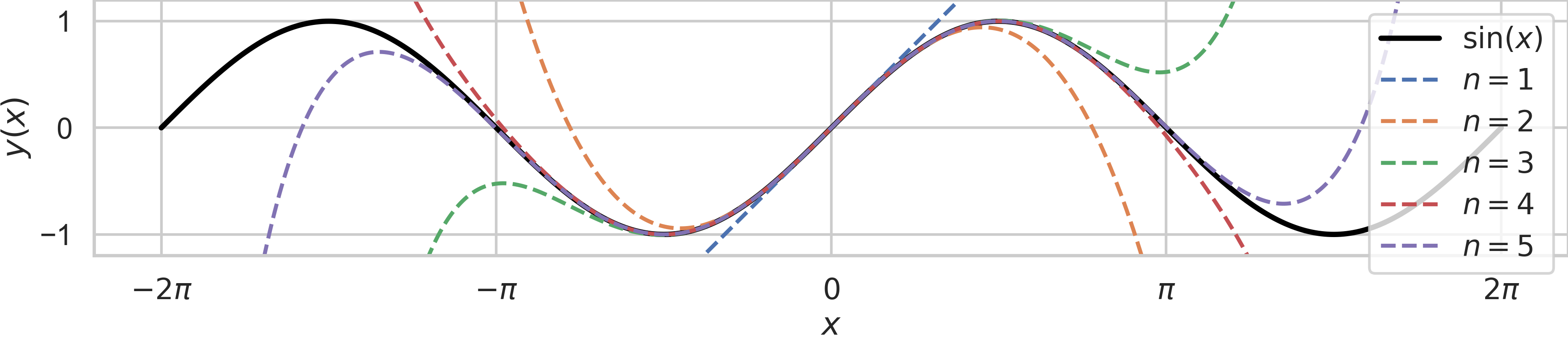
Fig. 13 Taylor series that approximates \(\sin(x)\) at \(x=0\) using \(1, 2, 3, 4, 5\) terms.

And we get

(15)\[\begin{split}\begin{split} \cos(t) &= T_{\cos(0)}(t) = \sum\limits_{k=0}^{\infty} \frac{\cos^{(k)}(0)}{k!}(t)\\ &= 1 - 0 - \frac{t^2}{2!} + 0 + \frac{t^4}{4!} - 0 - \frac{t^6}{6!} + \ldots \\ &= 1 - \frac{t^2}{2!} + \frac{t^4}{4!} - \frac{t^6}{6!} + \ldots \end{split}\end{split}\]

for the cosine function.

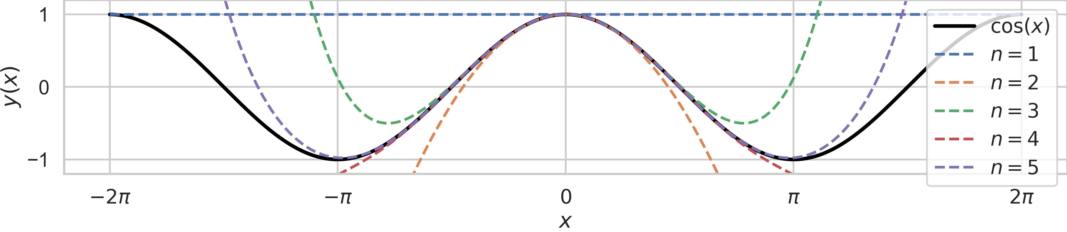
Fig. 14 Taylor series that approximates \(\cos(x)\) at \(x=0\) using \(1, 2, 3, 4, 5\) terms.

Furthermore, the natural exponential function has a quite nice form too, that is,

(16)\[\begin{split}\begin{split} e^t &= T_{e^0}(t) = \sum\limits_{k=0}^{\infty} \frac{\text{exp}^{(k)}(0)}{k!}t^k \\ &= \sum\limits_{k=0}^{\infty} \frac{t^k}{k!} \end{split}\end{split}\]

since \(\text{exp}^{(k)}(t) = \text{exp}(t)\) for all \(k \in \mathbb{N}_0\) and \(e^0 = 1\). Note that we donte \(e^t\) by \(\text{exp}(t)\).

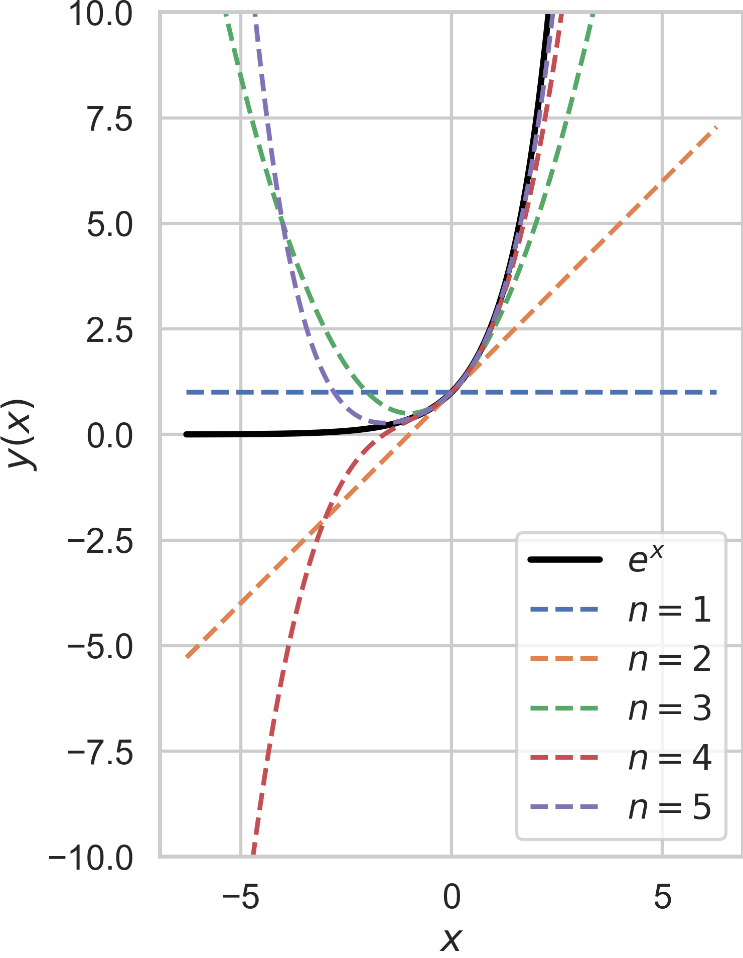
Fig. 15 Taylor series that approximates \(e^x\) at \(x=0\) using \(1, 2, 3, 4, 5\) terms.

What happens if we plug in an imaginary number like \(\phi i\), with \(\phi\in \mathbb{R}\)? Well let’s see:

\[\begin{split}\begin{split} e^{\phi i} &= T_{e^0}(\phi i) = \sum\limits_{k=0}^{\infty} \frac{(\phi i)^k}{k!}\\ &= 1 + \frac{\phi i}{1!} + \frac{\phi^2i^2}{2!} + \frac{\phi^3i^3}{3!} + \frac{\phi^4i^4}{4!} + \frac{\phi^5i^5}{5!} + \frac{\phi^6i^6}{6!} \ldots \\ &= 1 + \frac{\phi i}{1!} - \frac{\phi^2}{2!} - \frac{\phi^3i}{3!} + \frac{\phi^4}{4!} + \frac{\phi^5i}{5!} - \frac{\phi^6}{6!} - \ldots \\ &= \left( 1 - \frac{\phi^2}{2!} + \frac{\phi^4}{4!} - \frac{\phi^6}{6!} + \ldots \right) + i\left(\frac{\phi}{1!} - \frac{\phi^3}{3!} + \frac{\phi^5}{5!} - \ldots \right)\\ &= \cos(\phi) + i \sin(\phi). \end{split}\end{split}\]

We arrive at Euler’s formula which links the hyperbolic functions, involving \(e\), to trigonomeitric functions, involving \(\pi\)!

Euler’s Formula

Let \(i \phi\) be an imaginary number, then

(17)\[e^{i\phi} = \cos(\phi) + i \sin(\phi)\]

holds. This relation is called Euler’s formula.

exp(Complex(0, pi/3)) == Polar(1, pi/3).asComplex // true

We can immidiatly follow that

\[e^{i\pi} = \cos(\pi) + i \sin(\pi) = -1 + i0 = -1.\]

exp(Complex(0, pi)) + 1 < 0.00001  // true
exp(Complex(0, pi)) + 1 > -0.00001 // true

Therefore, the most beautiful formula of all times, called Euler’s identity, emerges

(18)\[\begin{equation} e^{i\pi} + 1 = 0. \end{equation}\]

Looking at Eq. (17) we immediately see that

(19)\[\begin{equation} \forall \omega \in \mathbb{R}: |e^{i \omega}| = 1 \end{equation}\]

holds. Therefore,

\[z = e^{i\omega} \Rightarrow |z^k| = 1.\]

I illustrate this fact by using \(z = e^{i \frac{2\pi}{N}}\), i.e. \(\omega = \frac{2\pi}{N}\) and the following plot, where the plotted points are defined by

\[z^k = e^{i \frac{2\pi}{N} k} \quad \text{ for } k = 0,1,2 \ldots, N-1 \text{ with } N=19.\]

All points lie on the red unit circle.

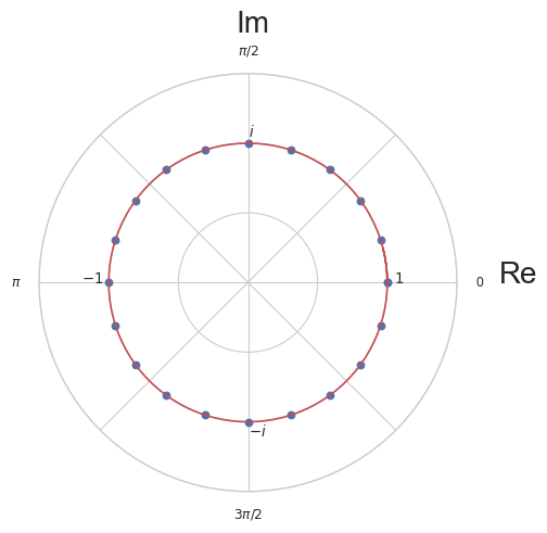
Furthermore, we can see that the discrete function \(g(k): \mathbb{Z} \rightarrow \mathbb{C}, \ g(z) = z^k\) is periodic and that its period is \(N\):

\[g(N+1) = \left( e^{i \frac{2\pi}{N}} \right)^{N+1} = e^{i \frac{2\pi (N+1)}{N}} = e^{i 2\pi} \cdot e^{i \frac{2\pi}{N}} = e^{i 0} \cdot e^{i \frac{2\pi}{N}} = 1 \cdot e^{i \frac{2\pi}{N}} = z = g(1).\]

If \(|z|\) would be greater than 1, then \(z^k\) would grow to infinity and if \(|z| < 1\), it would converge to \(0\).

Using Euler’s formula, i.e. Eq. (17), we can represent our well-known trigonometric functions by exponential functions. We start with

\[(\cos(\phi) + i\sin(\phi)) + (\cos(\phi) - i\sin(\phi)) = 2 \cos(\phi) = e^{i\phi} + e^{-i\phi}.\]

Therefore, we get

(20)\[\begin{equation} \cos(\phi) = \frac{e^{i\phi} + e^{-i\phi}}{2}. \end{equation}\]

For the sine, we start with

\[(\cos(\phi) + i\sin(\phi)) - (\cos(\phi) - i\sin(\phi)) = 2i \sin(\phi) = e^{i\pi} - e^{-i\pi}.\]

Therefore, we get

(21)\[\begin{equation} \sin(\phi) = \frac{e^{i\phi} - e^{-i\phi}}{2i} = -i\frac{e^{i\phi} - e^{-i\phi}}{2}. \end{equation}\]

Phasors

Interestingly, by using Euler’s formula, we can encode the phase and amplitude of a sinosoid by one very compact representation which we call phasor.

Phasor

A phasor is the polar representation of any complex variable

(22)\[\begin{equation} \hat{r}_\phi = r e^{i\phi}, \end{equation}\]

where \(r, \phi \in \mathbb{R}\). It represents the amplitude and phase shift of some sinosoid.

We can define any sinosoid of the form

(23)\[\begin{equation} y(t) = r \cdot \cos(2\pi f t + \phi) \end{equation}\]

using the only the real part of

(24)\[\begin{equation} \begin{split} \underbrace{\hat{r}_\phi}_{\text{phasor}} \cdot \underbrace{e^{i 2\pi f t}}_{\text{circular motion}} &= r e^{i\phi} \cdot e^{i 2\pi f t} = r e^{i (2\pi f t + \phi)}\\ &= r \cdot (\cos(2\pi f t + \phi) + i \sin(2\pi f t + \phi))\\ &= y(t) + i r \sin(2\pi f t + \phi)), \end{split} \end{equation}\]

where the phasor \(\hat{r}_\phi = r e^{i\phi}\) is a constant, \(f\) is the frequency, and \(\phi\) the phase of the sinusoid. The phasor \(\hat{r}_\phi\) tells us everything about the amplitude and the phase \(\phi\) of the signal \(y(t)\).

In many text books you will find

(25)\[\begin{equation} r e^{i (\omega t + \phi)} = r \cdot (\cos(\omega t + \phi) + i \sin(\omega t + \phi)) = y(t) + i r \sin(\omega t + \phi)) \end{equation}\]

instead, where \(\omega = 2\pi f\) is the anglar speed or speed of rotation.

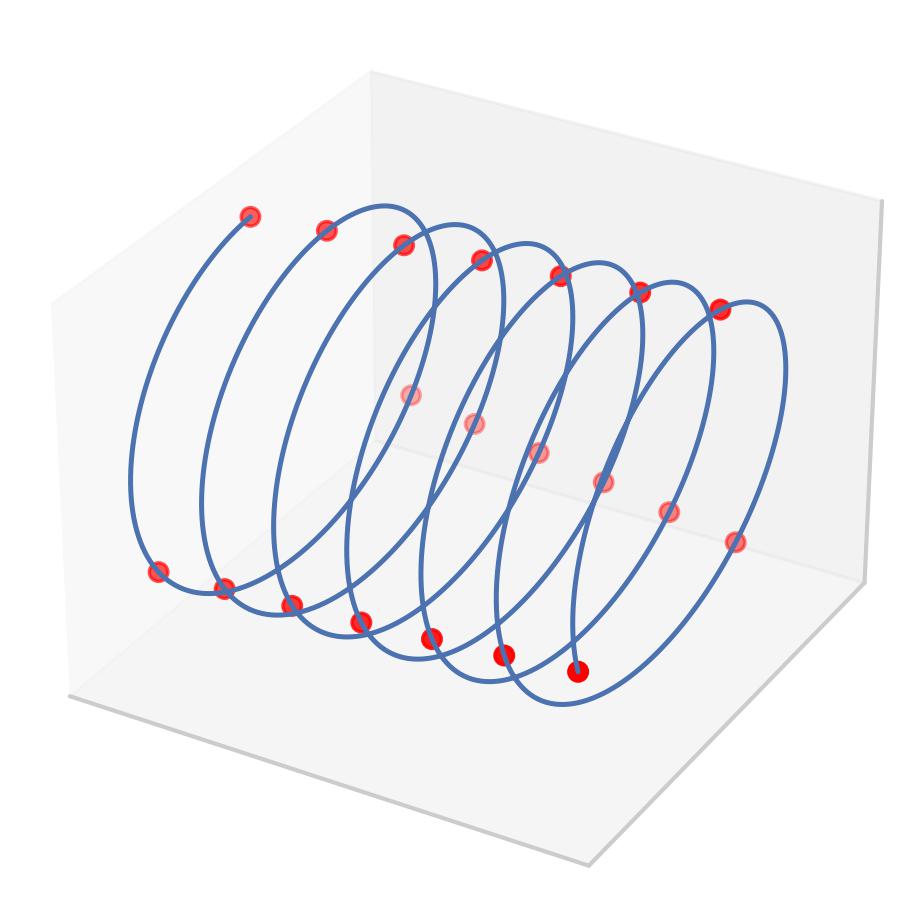
Fig. 16 A complex sinusoid \(y(t) = r e^{i (2\pi f t + \phi)}\). The phasor is the first red point, i.e. \(y(0)\).

Remember, we can represent any audio signal as a sum of sinusoids. Since each phasor is also a vector, a sinusoid comprising multiple frequencies can be represented as a sum of phasors.

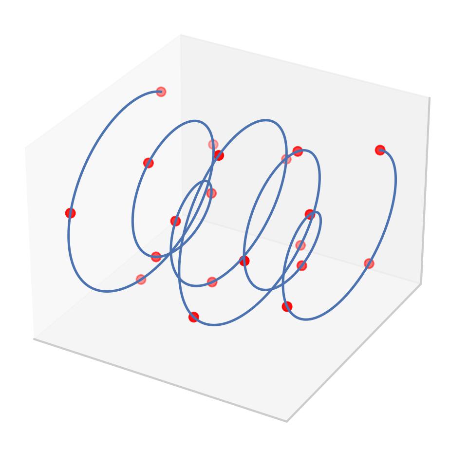
Fig. 17 A complex sinusoid \(y(t)\) defined by 3 phasors and 3 differen frequencies.