Amplitude Modulation#
If we modulate (change a value over time) the amplitude of an audible signal, we call this amplitude modulation (AM). We often speak of amplitude modulation when we modulate the amplitude within a value between 0 and 1 and use the term ring modulation if the modulator can also be negative. I put amplitude and ring modulation in the same basket.
As we will see, the frequency range of the modulation has a significant effect on the result. If it is low, e.g., in the range of 20 Hz, we call it low-frequency modulation. But first, let’s start with some math to understand better what is happening.
Theory#
I use the cosine function in this section instead of the sine because the math becomes a little simpler. Our basic waveform might be a simple cosine with an amplitude \(A(t)\) and a frequency \(f\):
In AM the amplitude \(A(t)\) is itself a function over time. Let us assume
then our audio signal is defined by
which we can rewrite as
We can now use the cosine rule for multiplication, which gives us
This looks complicated but if we look at the Fourier transformation of \(y(t)\), we can identify three frequencies within the spectrum:
the carrier frequency \(f_\text{car}\) with an amplitude \(A_\text{car}\),
the sum of the carrier and modulation frequency \(f_\text{car} + f_\text{mod}\) with an amplitude of \(1/2 \cdot A_\text{mod}\) and
the difference of the carrier and modulation frequency \(f_\text{car} - f_\text{mod}\) with an amplitude of \(1/2 \cdot A_\text{mod}\).
Effect#
If the modulation frequency is low, that is, in the range of \(0\) and \(20\) Hz, we can recognize an amplitude modulation by the change of amplitude in \(y(t)\). However, if we choose a modulation frequency in the range of audible frequencies, we no longer really modulate the amplitude of the signal \(y(t)\) but the frequencies of the signal.
For example, if we use \(A_\text{car} = A_\text{mod} = 1\) and \(f_\text{car} = 400\) Hz, \(f_\text{mod} = 250\) Hz, the signal consists of three frequencies:
\(400\) Hz (center)
\(400 + 250 = 650\) Hz (sum) and
\(400 - 250 = 150\) Hz (difference), compare Fig. 62.
We can listen to this effect using the following code:
(
Spec.add(\freq, [100, 600]);
Spec.add(\freqmod, [0.01, 600]);
Spec.add(\ampcar, [0, 1]);
Spec.add(\ampmod, [0, 1]);

Ndef(\am, {
    var sig, amp;
    amp = \ampcar.kr(1) + (\ampmod.kr(1) * SinOsc.ar(
            \freqmod.kr(5),
            0.5*pi)
        );
    sig = SinOsc.ar(\freq.kr(200), 0.5*pi);
    sig = sig * amp * (1/3) ! 2;
}).play;
)

Ndef(\am).gui
Try out different values and observe the resulting sound.
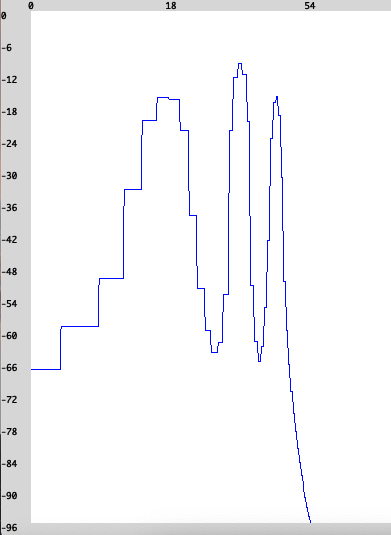
Fig. 62 Snapshot of the stethoscope using a logarithmic frequency scale (\(x\)-axis). I use \(A_\text{car} = A_\text{mod} = 1\) and \(f_\text{car} = 400\) Hz, \(f_\text{mod} = 250\) Hz.#
Techniques#
In our example above, we used a fixed modulation frequency, i.e., if we change the carrier frequency the modulation frequency stays constant.
Direct Current#
If we use, for example, \(f_\text{car} = f_\text{mod} = 100\) Hz we achieve frequencies equal to \(0\), \(100\) and \(200\) Hz. Zero means no oscillation which results in an offset (\(y\)-axis) of the signal. We call this a DC (direct current).
The following code generates a plot, such that you can observe this effect.
({
    var sig, amp;
    amp = \ampcar.kr(1) + (\ampmod.kr(1) * SinOsc.ar(\freqmod.kr(100), 0.5*pi));

    sig = SinOsc.ar(\freq.kr(100), 0.5*pi);
    sig = sig * amp * (1/3);
    sig
}.plot(1/100))
The result is depicted in Fig. 63. All values \(y(t)\) are shifted up, that is, in positive \(y\)-direction.
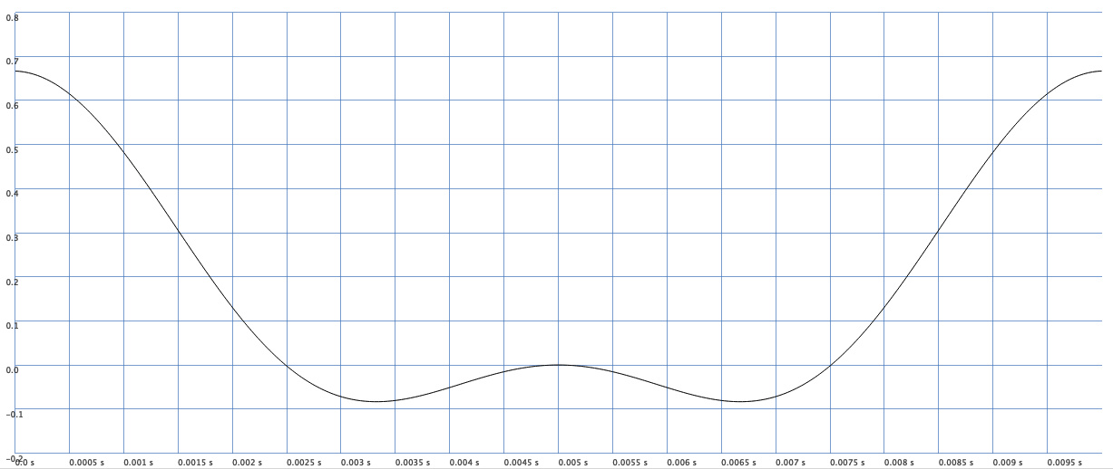
Fig. 63 DC (direct current) results in an offset of the signal.#
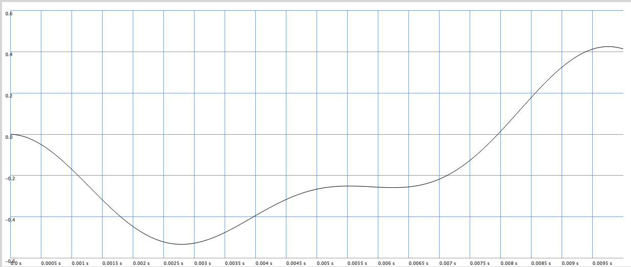
This effect can be avoided by using the LeakDC unit generator which tries to center a signal on the amplitude-axis.
({
    var sig, amp;
    amp = \ampcar.kr(1) + (\ampmod.kr(1) * SinOsc.ar(\freqmod.kr(100), 0.5*pi));

    sig = SinOsc.ar(\freq.kr(100), 0.5*pi);
    sig = sig * amp * (1/3);
    sig = LeakDC.ar(sig);
    sig
}.plot(1/100))
gives
Clangoros Sound#
When we play different notes by adjusting the carrier frequency without altering the modulation frequency, we achieve a non-harmonic, clangorous sound. The relationship between the frequencies maintains a fixed offset, meaning that for a high carrier or central frequency, the sum and difference frequencies are closer to the center frequency compared to those at lower center frequencies.
Across nearly all carrier frequencies, harmonics are absent from the signal. This inharmonicity results in a distinctly clangorous sound. It can be utilized to generate aggressive and conventionally “unmusical” sounds that shift dramatically as one progresses up and down the keyboard.
We can control the amount of clangor by raising or lowering the level of the modulator \(A_\text{mod}\).
Harmonic and Inharmonic Timbres#
Let us introduce a ratio \(r\) between the carrier frequency and the modulation frequency such that:
which results in frequencies \(f_\text{car}\) and
\(r\) should be smaller or equals than \(1\).
(
Spec.add(\freq, [100, 600]);
Spec.add(\ratio, [0.0, 10]);
Spec.add(\ampcar, [0, 1]);
Spec.add(\ampmod, [0, 1]);

Ndef(\am, {
    var sig, amp, freqmod;
    freqmod = \radio.kr(1) * \freq.kr(200);
    amp = \ampcar.kr(1) + (\ampmod.kr(1) * SinOsc.ar(freqmod, 0.5*pi));

    sig = SinOsc.ar(\freq.kr(200), 0.5*pi);

    sig = sig * amp * (1/3) ! 2;
}).play;
)
We get a harmonic relationship if the ratio is an integer, but this is a special case! In general, the relationship is inharmonic, and we increase the inharmonicity if we use a ratio far away from a whole number!
Remember, the frequencies the signal has are \((1 \pm r) \cdot f_\text{car}\) and \(f_\text{car}\). So the coefficients in order they are:
For example, this gives us:
\(r=1/4\): \(3/4, 1, 5/4\)
\(r=1/2\): \(1/2, 1, 3/2\)
\(r=1/1\): \(0, 1, 2\)
\(r=2/1\): \(-1, 1, 3\)
\(r=3/2\): \(-1/2, 1, 5/2\)
…
Unipolar Amplitude Modulation#
We speak of unipolar if the modulation signal either stays positive or negative over time. For example:
({
    var mod = SinOsc.ar(110, mul: 0.5, add: 0.5);
    var car = mod * SinOsc.ar(440);
    car;
}.play;
)
The effect is very similar.
Complex Amplitude Modulation#
Instead of using sine waves we can also use other signals, for example we could use for one or both of the signals (carrier and modulator) a sawtooth wave. If the carrier signal consists of frequencies equal to \(f_{\text{car},1}, \ldots, f_{\text{car},n}\) and the modulator consists of frequencies \(f_{\text{mod},1}, \ldots, f_{\text{mod},m}\), then the resulting signal will consist of frequencies:
thus it consists of \((n+1) \cdot m\) frequencies (if nothing cancels out). Consequently, AM can generate complex signals with a rich frequency spectrum in a computational inexpensive way.
({
    var mod = LFSaw.ar(110);
    var car = mod * LFSaw.ar(200);
    car = car * 0.25;
    LeakDC.ar(car!2);
}.play;
)
car consists of frequencies of all harmonics of the carrier \(200, 400, \ldots\) combined with all harmonics of the modulator \(110, 220, 330, \ldots\).
If we would use \(100\) Hz for the fundamental of the modulator, the result would be a signal that does only contain odd harmonics.
({
    var mod = LFSaw.ar(100);
    var car = mod * LFSaw.ar(200);
    car = car * 0.25;
    LeakDC.ar(car!2);
}.play;
)
If we use low modulation frequency, we can achieve some distortion. The following sounds a bit like the sound of a helicopter.
({
    var mod = LFSaw.ar(LFNoise1.ar(1).range(10, 15));
    var car = mod * LFSaw.ar(200);
    car = LPF.ar(car, 500);
    car = car * 0.25;
    LeakDC.ar(car!2);
}.play;
)