Harmonic Series

Let us recreate or approximate the sawtooth wave without using the LFSaw or Saw unit generator. Instead, we use a bunch of SinOsc oscillators. This gives us full control over the amplitude of each frequency, i.e. full control over the power distribution.

The following code generates the sound of the Fourier series approximation. I implemented Eq. (51). You can change n to increase the number of harmonics that are present in the sound.

(
Ndef(\saw_approx, {
    var sig, amp=0.5, n=10, harmonics;
    harmonics = Array.geom(n, 1, -1) * Array.series(n, 1, 1);

    sig = harmonics.collect({ arg k;
        SinOsc.ar(\freq.kr(220)*abs(k)) / k;
    }).sum;
    sig = (1/pi) * sig!2 * amp;
}).play;
)

Client vs Sever

We are tempted to convert the variable n into an argument that we can change while the synth is playing! Here we enter the limits of a synth or, in other words, the difference between sclang and the code running on the audio server.

sclang is executed on the client. Therefore, the do-construct is executed on the client before the synth definition is sent to the server. In some sense, the synth definition is compiled, and n is a variable that is fixed at run time. Consequently, changing n while the synth is playing will not change anything.

My machine has no problem running over hundred oscillators (n=100). The CPU workload is at about 8-9 percent. If we only use the first ten harmonics, the sound is much more doll, and it becomes crispier by adding more and more harmonics. However, for me, at least, at some point, it is hard to perceive any difference if I add even more harmonics.

Ok, so far so good. Of course, it makes no real sense to recreate the pure sawtooth wave by multiple oscillators because it is much more computational expensive. But if we introduce modulation we can create many different sounds that can not be produced by only one sawtooth wave. Even with filters this can be quite challenging or impossible.

For example, a string of a perfect violin makes a sound that can be described by a sawtooth wave – each harmonic of the fundamental is present. However, there is no globally determining envelope. Instead, each frequency changes its power over time independently. This gives the violin its distinct timbre. A real violin sounds completely different than a sawtooth wave combined with an envelope. Furthermore, the world is imperfect, and so is the violin – there is always some distortion, also within the frequencies. Fortunately, our ears like this slight imperfection. By introducing imperfections, the sound becomes more gentle. It is a balance between order and chaos. In summary, for a real violin

1. the amplitudes of the harmonics deviate from Eq. (51),

2. they slightly deviate over time – each in a different way,

3. and their power (amplitude) is a unique function of time.

Adding a Global Envelope

Let is first try a percussive envelope: The sound is quite boring because nothing changes over time. There is no dynamic thus our ears lose interest immediately.

(
Ndef(\saw_approx, {
    var sig, amp=0.5, n=20, env, harmonics;

    env = EnvGen.ar(Env.perc(
        attackTime: \attk.kr(0.1),
        releaseTime: \rel.kr(1.0),
        curve: \curve.kr(-4)),
    doneAction: Done.freeSelf
    );

    harmonics = Array.geom(n, 1, -1) * Array.series(n, 1, 1);

    sig = harmonics.collect({ arg k;
        SinOsc.ar(\freq.kr(220)*abs(k)) / k;
    }).sum;
    sig = (1/pi) * sig!2 * amp * env;
}).play;
)

Let us introduce some change over time.

Dynamic Frequency Detuning

To bring in some movement, we want to change frequencies over time. This is called frequency modulation, but we only want to change the frequency very slightly. There are an infinite amount of strategies to do this. A straightforward way is to use a random number generator. I make use of LFNoise1. It chooses a value between 1 and -1 every \(1/f\) seconds where \(f\) is its frequency. In between these times, values are linearly interpolated.

I introduce a LFNoise1 for each harmonic. It generates values between \([1-\epsilon; 1+\epsilon]\). Note that for each speaker, the noises are different! It is hard to explain what exactly happens with our vibrato over time so let us plot an example.

{LFNoise1.ar(100!2).range(1-0.015, 1+0.015)}.plot(1.01)

gives us the following plot:

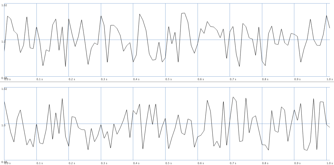
\(\epsilon\) is the percentage of maximal detune, i.e., a harmonic with a frequency of \(f\) will have an actual frequency within

\[[f \cdot (1-\epsilon); f \cdot (1+\epsilon)].\]

In the code below, I call \(\epsilon\) detune. The detune changes over time. The updated version of \sine_sum looks like the following:

(
Ndef(\saw_approx, {
    var sig, amp=0.5, n=20, env, harmonics;
    var detuneFreq = 5;
    var detune = 0.015;

    harmonics = Array.geom(n, 1, -1) * Array.series(n, 1, 1);

    env = EnvGen.ar(Env.perc(
        attackTime: \attk.kr(0.01),
        releaseTime: \rel.kr(1.0),
        curve: \curve.kr(-4)),
    doneAction: Done.freeSelf
    );

    sig = harmonics.collect({ arg k;
        var vibrato = LFNoise1.ar(detuneFreq!2).range(1-detune, 1+detune);
        var harmonicFreq = \freq.kr(220) * vibrato * abs(k);
        SinOsc.ar(harmonicFreq) / k;
    }).sum;

    sig = (1/pi) * sig * amp * env;
}).play;
)

In my opinion, this already sounds much more interesting. Of course, we went beyond additive synthesis and used frequency modulation but those go hand in hand, especially if the modulation frequency is low.

Individual Envelopes

What can we do in addition? Well, at the moment, we have one global envelope for all frequencies. What about n independent envelopes? We could, for example, imitate nature and decrease the amplitudes of high frequencies faster than those of low frequencies. We could introduce randomness such that only the expected decrease in amplitude behaves like that.

(
SynthDef(\saw_approx, {
    var sig, n=20, harmonics;

    harmonics = Array.geom(n, 1, -1) * Array.series(n, 1, 1);

    sig = harmonics.collect({ arg k;
        var env = EnvGen.ar(Env.perc(
            attackTime: \attk.kr(0.01) * Rand(0.8,1.2),
            releaseTime: \rel.kr(5.0) * Rand(0.9,1.1),
            curve: \curve.kr(-4))
        );

        var vibrato = 1 + LFNoise1.ar(\detuneFreq.kr(5)!2).bipolar(\detune.kr(0.015));
        var harmonicFreq = \freq.kr(220) * vibrato * abs(k);
        (1/pi) * SinOsc.ar(harmonicFreq) / k * env.pow(1+((abs(k)-1)/3));
    }).sum;

    sig = LPF.ar(sig, 1500);
    sig = sig * \amp.kr(0.5);
    DetectSilence.ar(sig, doneAction: Done.freeSelf);
    Out.ar(0, sig);
}).add;
)

Synth(\saw_approx);

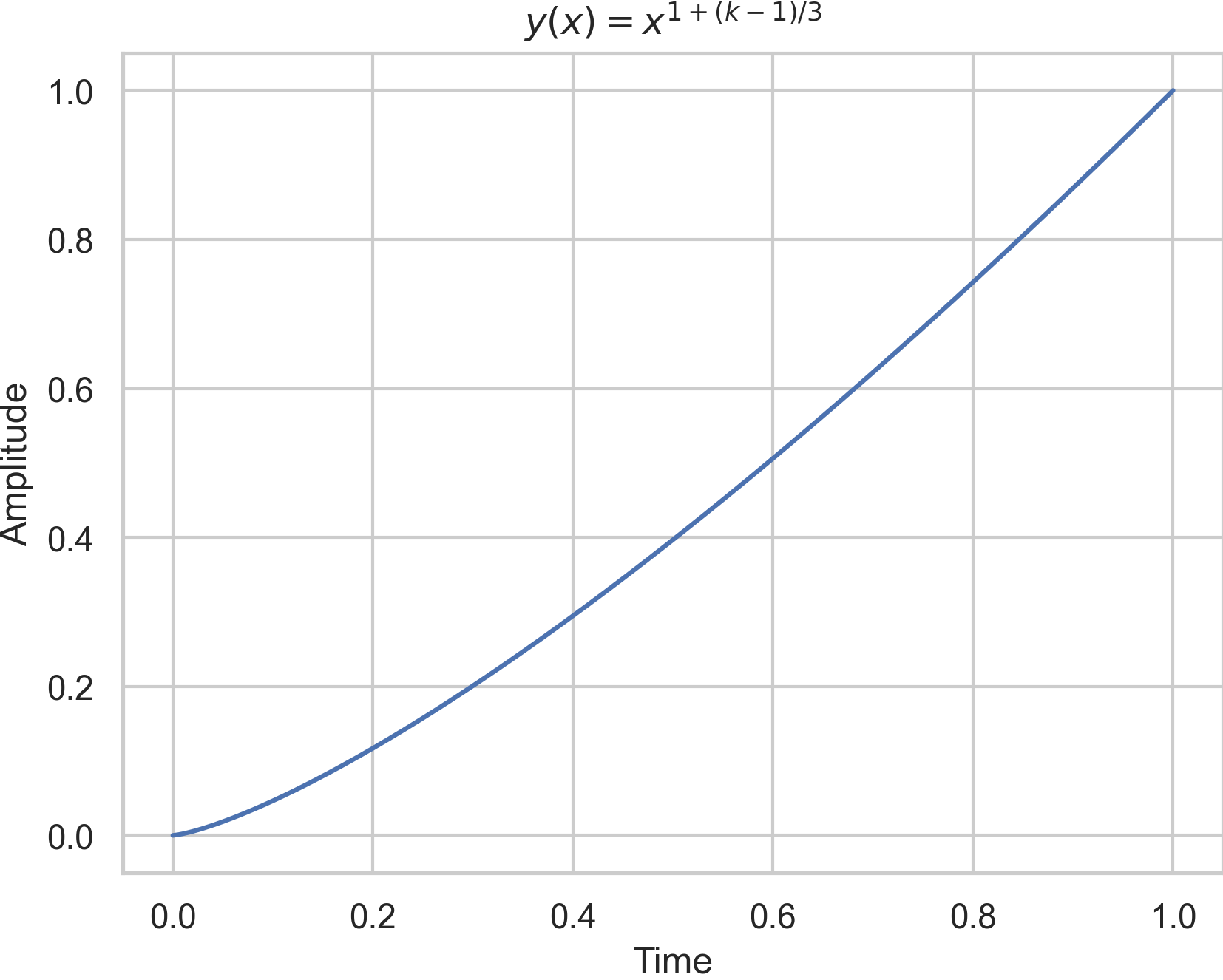
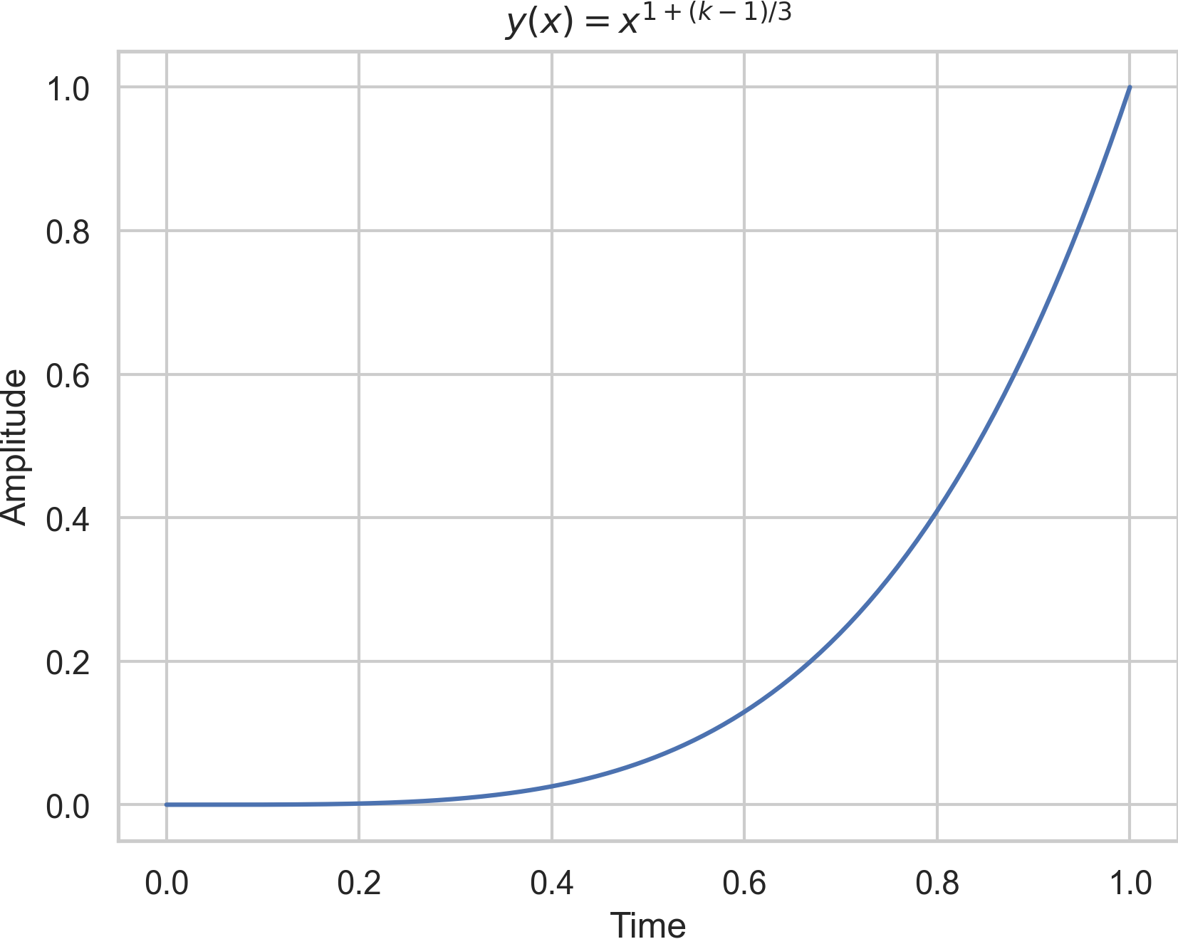
Ok, this doesn’t look very easy. However, I did not change too much. First, I have rewritten the series such that the sum is the most outer operation. Secondly, I generate for each frequency one independent envelope with a random attack and release. Thirdly, I use a neat trick to decrease the envelope for high frequencies faster: I take power

(58)\[ x \leftarrow x^{1 + \frac{k-1}{3}}\]

where \(x\) is a value of the envelope (a series of numbers) of the \(k^\text{th}\)-harmonic. Compare the following two plots.

Fig. 45 The effect of Eq. (58) for \(k = 2\).

Fig. 46 The effect of Eq. (58) for \(k = 10\).

Fourthly, I removed the doneAction: Done.freeSelf from the envelopes because this would shut down the synth as soon as the first envelope reached its end. The sound would abruptly end too early. To clean up the audio server, I use DetectSilence-UGen instead. It executes the cleanup, that is, the action freeSelf if the signal sig indicates silence for a short period, which is very handy.

Let’s finally create a discrete musical event simulation:

(
Pbindef(\melody,
    \instrument, \saw_approx,
    \dur, Pshuf(2.pow((-4..1)), inf),
    \rel, 6.0,
    \detune, Pwhite(0.001, 0.01, inf),
    \detuneFreq, 20,
    \amp, 0.3,
    \octave, Pdup(Prand([2,3,4], inf), Pseq([3,4,5], inf)),
    \degree, Pshuf([0, 2, 5, 6, 8, 11], inf),
).play;
)

Changing the Power Distribution

The amplitudes of each harmonic overtone still mirrows the amplitude of its counterpart in a sawtooth wave. We can further individualize the sound by changing this. We can easily choose individual frequencies, amplitudes and phases.

In the following I use, aside from the fundamental, the 3., 5., 6., 7., 8. and 9-th harmonics. You can play the pattern while changing the amplitudes and the number of each harmonic to alter the sound. You can also add addtional harmonics.

(
SynthDef(\sine_sum, {
    var sig, harmonics, amps, phases;

    harmonics = [1, 3, 5, 6, 7, 8, 9];
    phases = [0, 0, 0, 0.5, 0.25, 0, 0] * 2*pi;
    amps = [0.5, 0.1, 0.2, 0.6, 0.6, 0.1, 0.1].normalizeSum();

    sig = harmonics.collect({ arg k, index;
        var env = EnvGen.ar(Env.perc(
            attackTime: \attk.kr(0.01) * Rand(0.8,1.2),
            releaseTime: \rel.kr(5.0) * Rand(0.9,1.1),
            curve: \curve.kr(-4))
        );

        var vibrato = 1 + LFNoise1.ar(\detuneFreq.kr(5)!2).bipolar(\detune.kr(0.015));
        var harmonicFreq = \freq.kr(220) * vibrato * abs(k);
        amps[index] * SinOsc.ar(harmonicFreq, phases[index]) / k * env.pow(1+((abs(k)-1)/3));
    }).sum;

    sig = LPF.ar(sig, 1500);
    sig = sig * \amp.kr(0.5);
    DetectSilence.ar(sig, doneAction: Done.freeSelf);
    Out.ar(0, sig);
}).add;
)