Fourier Series

L’étude profonde de la nature est la source la plus féconde de découvertes mathématiques. – Jean-Baptiste Joseph Fourier (1768–1830)

Given a signal \(y(t)\) of a played piano key, how can we compute the pitch, and how can we recreate that sound? Spectral analysis and synthesis give us some answers. By transforming the representation of a signal, we can catapult ourselves from the space of amplitude over time into the space of intensity over frequencies.

In mathematics, the meaning of transform and transformation is somewhat specific, but it still is relatively wide or loose when the definition sometimes says it is a mathematical quantity obtained from a given quality by an algebraic, geometric, or functional operation. In transform theory, mathematicians talk about a suitable choice of a function called kernel (from the German nucleus or core), by which a problem may be simplified.

In 1822 Jean-Baptise Joseph Fourier discovered a truly remarkable transformation which gives us insights into our knowledge of waveforms in general and music in particular. He claimed that any function, whether continuous or discontinuous, can be transformed into a series of sines. That important work was corrected to

almost any periodic function can be represented by a Fourier series that converges.

and expanded upon by others to provide the foundation for various forms of the Fourier transform used since.

I find this result still fascinating. At this point, I have to mention that the great German mathematician Carl Friedrich Gauß already discovered this connection in 1805 and, what is even more remarkable, he formulated something quite similar to the fast Fourier transform (FFT)! His breakthrough was not widely adopted because it only appeared after his death in volume three of his collected works which was written with non-standard notation in a 19th-century version of Latin.

Especially since the re-discovery of the fast Fourier transform (FFT) in 1965 by Cooley and Tukey to detect underground tests of atomic bombs, the Fourier synthesis is a widespread technique performed in all areas of signal processing. There are so many applications of the FFT, from solving differential equations to radar and sonar, studying crystal structures, WiFi, and 5G. It is no surprise that the mathematician Gilbert Strang called the FFT

the most important numerical algorithm of our lifetime. – Gilbert Strang

But why is that? Well, it is all about computation speed! The FFT reduces the time complexity of the discrete Fourier transformation (DFT) from \(\mathcal{O}(n^2)\) to \(\mathcal{O}(n\log(n))\) which makes the computation of the DFT fast thus applicable for many areas and purposes.

Frequency Spectrum

Before we dicuss the mathematical basis, let’s have a look at the frequency spectrum of a audio recordings such that we can picture what we want to compute. First let us use an audio recording of a physical piano. The note played is A0 = 440 Hz.

We can display the waveform of the signal

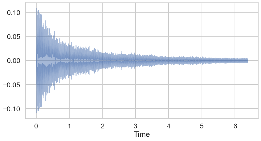
Fig. 18 Waveform, i.e., the audio signal in the time domain.

as well as the frequency sprectrum

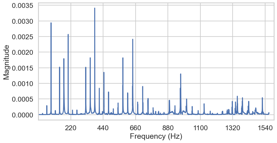
Fig. 19 Fourier coefficients, i.e., the audio signal in the frequency domain.

The spectrum is computed by the discrete Fourier transform. As you can see, there are even lower frequencies than the fundamental present and the signal consists of a lot inharmonic content. The piano might be out of tune.

Let us look at a second synthetic example:

The sound was generated by the following code.

({
    var sig = SinOsc.ar(440 * [1,2,3,4,5]) * [0.5, 0.2, 0.2, 0.1, 0.1];
    sig = Mix(sig);
    [sig, sig];
}.play;)

We can display the wave form of the signal (here I only plot a very short time period)

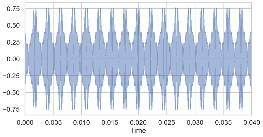
Fig. 20 Synthetic waveform, i.e., the audio signal in the time domain.

as well as the frequency sprectrum

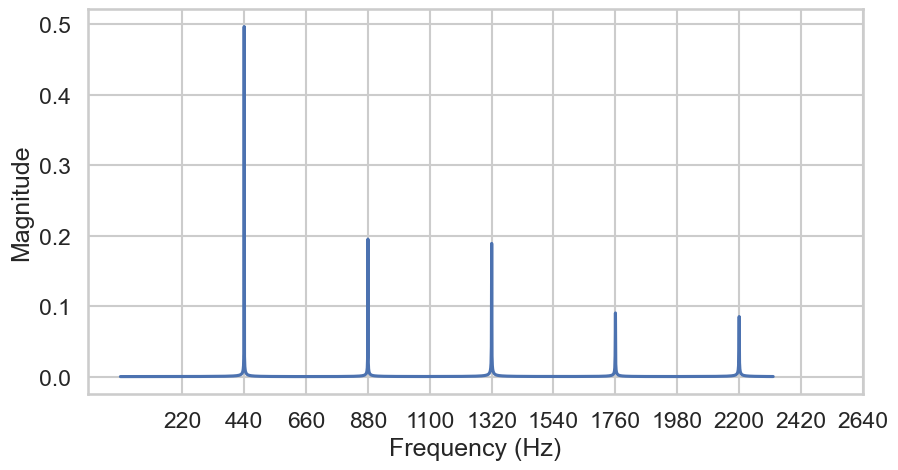
Fig. 21 Synthetic Fourier coefficients, i.e., the audio signal in the frequency domain.

In the synthetic case, we get exaclty what we expected, i.e., 5 peaks, four harmonic overtones, and one fundamental at 440 Hz.

Similarity of Periodic Functions

Let us start from the assumption that the Fourier theorem is correct (which it is). So we assume, that we can built any periodic vibration using a combination of sinusiods whose frequencies are integer multiple of a fundamental frequcency. Our job is to find the correct amplitudes and phases of these sinusiods. Let’s ignore the phase for a moment. We assume that all phases are zero.

The question that we have to answer is: how much of a specific sinusoidal is in \(y(t)\). If the answer is a lot, then the amplitude of the respective sinosoid should be large. Therefore, computing sinusoidals that are similar to \(y(t)\) seems to be a good starting point. Instead of similarity one speaks of cross-correlation which is a measure of similarity of two series as a function of the displacement of one relative to the other, also known as sliding dot product or sliding inner-product.

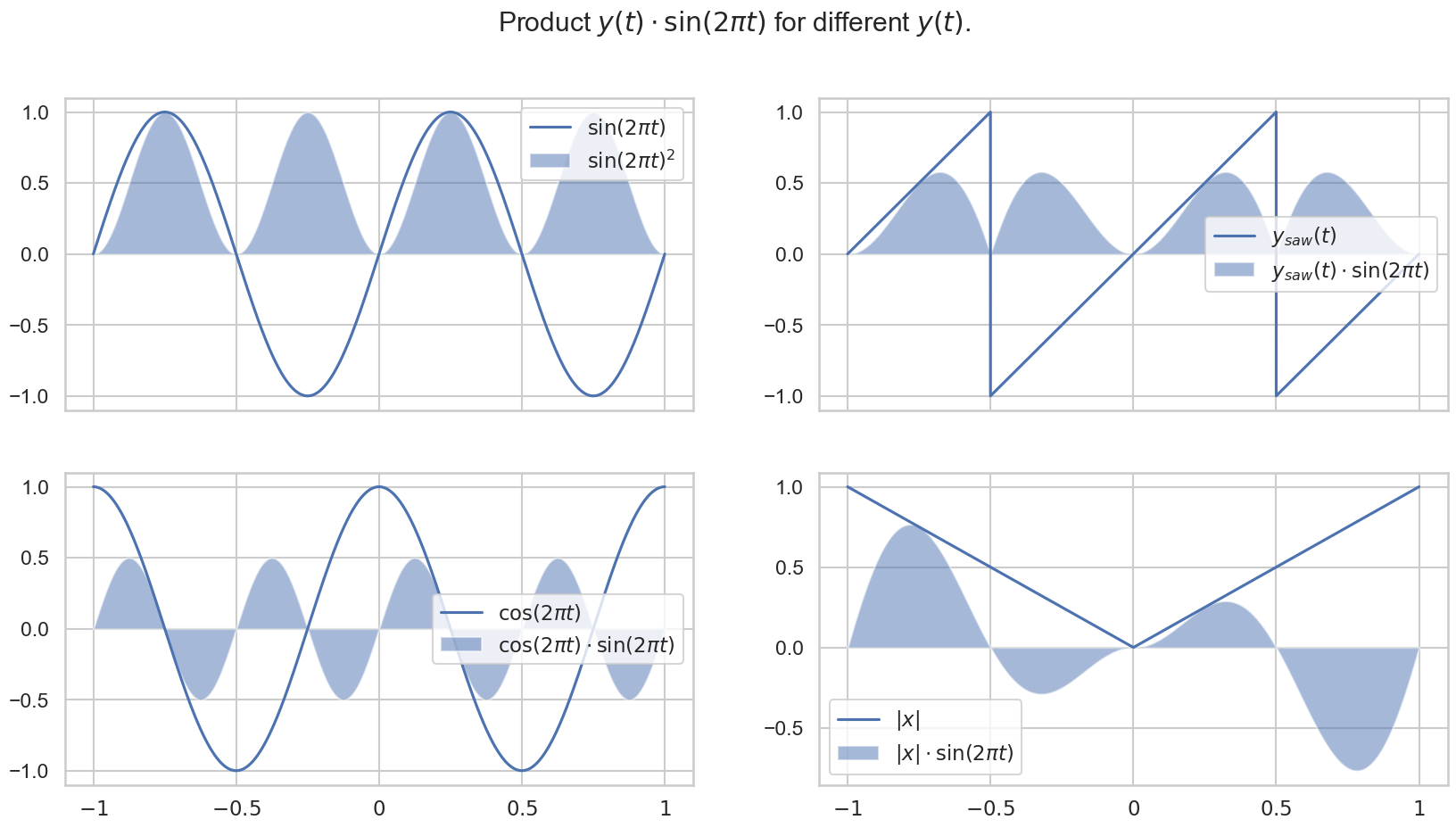
Functions are similar if their product result in a positive function. In other words, if the integral of their product is positive.

In the following plot we can see this intuition at play. The integral of \(\sin(2\pi t)^2\) gives us \(0.5\), i.e., there is alot of \(\sin(2\pi t)\) in \(\sin(2\pi t)\). We also get a positive value for the integral of \(\sin(2\pi t)\) multiplied with the sawtooth wave. The integrals of the other products are zero.

( // generate the y(t) * sin(2*pi*u)
{[
    SinOsc.ar(1) * SinOsc.ar(1), 
    LFSaw.ar(1) * SinOsc.ar(1),
    SinOsc.ar(1) * SinOsc.ar(1,0.5*pi),
    LFTri.ar(0.5)*(-1)*SinOsc.ar(1)
]}.plot(1)
)

Let’s have a look at the sum of the first terms of the sawtooth wave:

\[y(t) = \sum_{k=1}^8 \frac{1}{k}\sin(2\pi \cdot k \cdot t).\]

For shorthand let us also define the product with a sine wave of a certain frequency of \(n \in \mathbb{N}\) Hz:

\[g_n(t) = y(t) \cdot \sin(2\pi \cdot n \cdot t).\]

({
    var sines = Array.fill(8, {arg i; 1/(i+1) * SinOsc.ar(i+1);});
    var y = Mix(sines);
    [y]++Array.fill(8, {arg i; y*SinOsc.ar(i+1)});
}.plot(1)
)

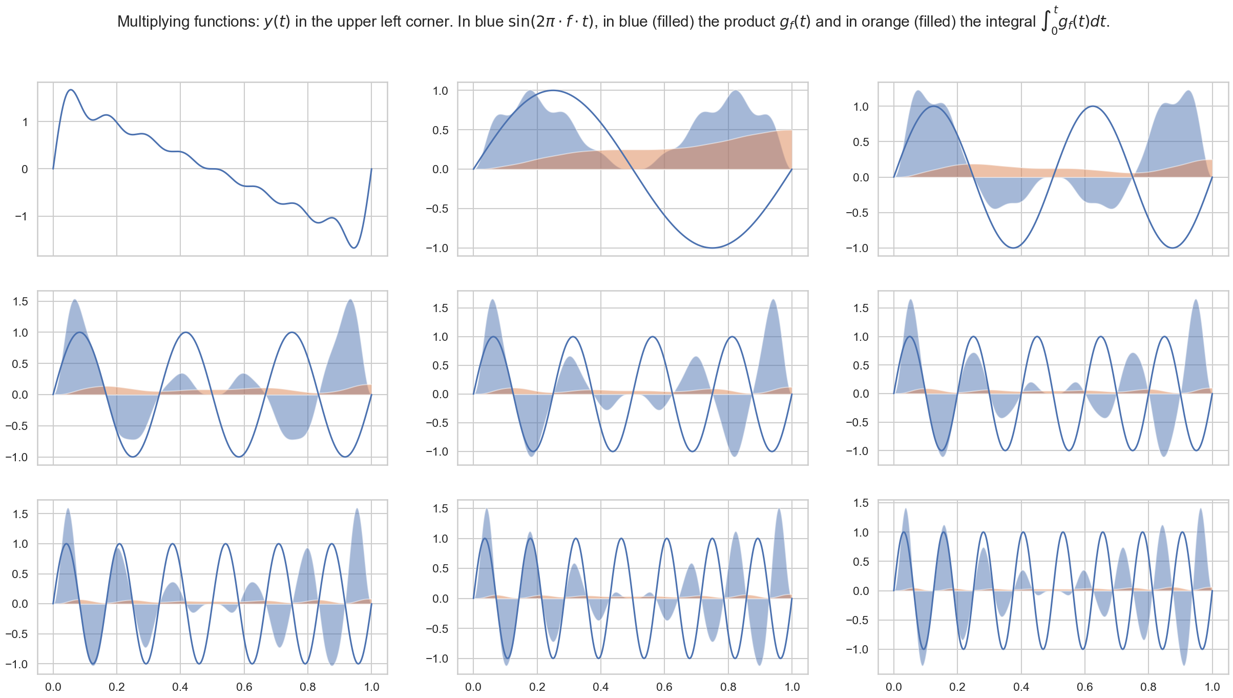
We get

\[\int_0^1 g_1(t)dt = \frac{1}{2}, \int_0^1 g_2(t)dt = \frac{1}{4}, \int_0^1 g_3(t)dt = \frac{1}{6}, \int_0^1 g_4(t)dt = \frac{1}{8}, \ldots\]

In general we get

\[ \int_0^1 g_n(t)dt = \frac{1}{2n}.\]

Note that \(\forall n \in \mathbb{N}:\)

\[\int_0^1 \sin(2\pi \cdot n \cdot t)^2 dt = \frac{1}{2}\]

holds, thus

\[\int_0^1 \frac{1}{n}\sin(2\pi \cdot n \cdot t)^2 dt = \frac{1}{n} \int_0^1 \sin(2\pi \cdot n \cdot t)^2 dt = \frac{1}{2n}.\]

Therefore,

\[\int_0^1 g_n(t) dt = \frac{1}{n}\int_0^1 \sin(2\pi \cdot n \cdot t)^2 dt\]

follows. If we look at the integral of

\[h_n(t) = \left( y(t) - \frac{1}{n}\sin(2\pi \cdot n \cdot t) \right) \cdot \sin(2\pi \cdot n \cdot t),\]

then \(\forall n \in \mathbb{N}:\)

\[\int_0^1 h_n(t) dt = \int_{-\infty}^\infty h_n(t) dt = 0\]

holds. In fact, if we look at \(h_{i,j}(t) = \sin(2\pi i \cdot t ) \cdot \sin(2\pi j \cdot t)\)

(26)\[\begin{split}\begin{split} \forall i, j \in \mathbb{N}, i \neq j: \int_0^1 h_{i,j}(t) dt &= \int_{0}^1 h_{i,j}(t) dt = 0\\ &= \int_{-\infty}^\infty \sin(2\pi i \cdot t) \cdot \sin(2\pi j \cdot t ) dt\\ &= \int_{-\infty}^\infty h_{i,j}(t) dt \end{split}\end{split}\]

holds.

Perpendicular Functions

For all frequencies \(i, j \in \mathbb{N}\) with \(i \neq j\)

\[\int_0^1 \sin(2\pi i \cdot t) \cdot \sin(2\pi j \cdot t ) dt = \int_{-\infty}^\infty \sin(2\pi i \cdot t) \cdot \sin(2\pi j \cdot t ) dt= 0\]

holds. We say that \(\sin(2\pi i \cdot t)\) is perpendicular to \(\sin(2\pi j \cdot t)\).

({ // generate sin(2*pi*i*x) * sin(2*pi*j*x)
    var sines = Array.fill(3, {arg i; 1/(i+1) * SinOsc.ar(i+1);});
    var y = Mix(sines);
    var indices = Array.fill2D(3, 3, {arg row, col; [row,col];}).flatten;
    indices.collect({arg index; var i = index[0], j = index[1];
        SinOsc.ar(i+1)*SinOsc.ar(j+1)
    });
}.plot(1)
)

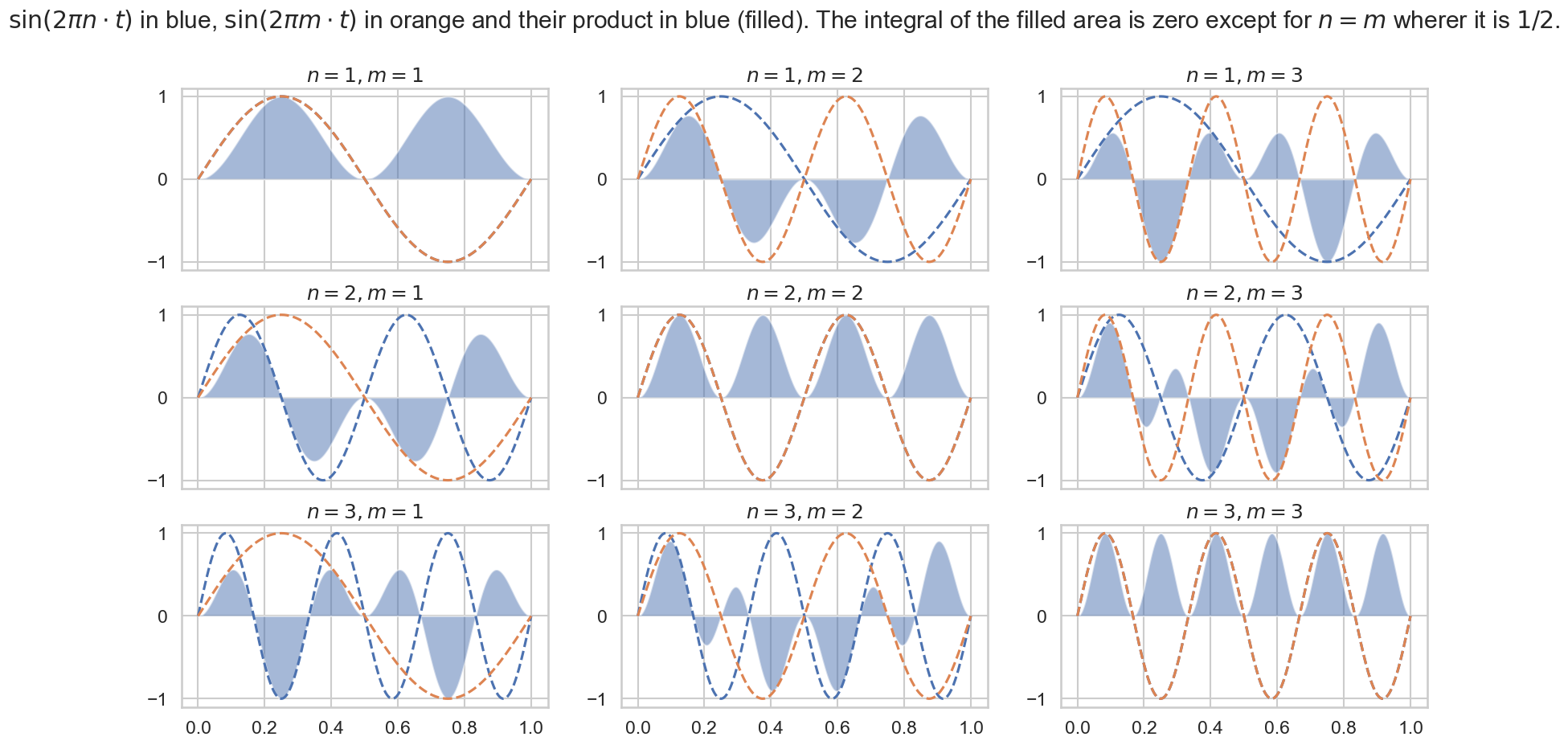
We say that these functions are perpendicular to each other because their scalar product (the integral of their product) is zero!

The similarity measure of two functions is similar to the similarity of two vectors. One way to compare two vectors \(\mathbf{a} = (a_1, \ldots, a_n)\) and \(\mathbf{b} = (b_1, \ldots, b_n)\) is to compute their inner product. If two vectors \(\mathbf{a}, \mathbf{b}\) are perpendicular, i.e., if they are very different, their inner product

\[<\mathbf{a}, \mathbf{b}> := \sum\limits_{i=1}^n a_i \cdot b_i\]

is zero. Their inner product is large if they are similar. We can define the inner product of two functions \(h: \mathbb{R} \rightarrow \mathbb{R}\) and \(g: \mathbb{R} \rightarrow \mathbb{R}\) in a similar fashion. The sum changes to an integral.

Inner Product of two Functions

Let \(h: \mathbb{R} \rightarrow \mathbb{R}\) and \(g: \mathbb{R} \rightarrow \mathbb{R}\) then

(27)\[ <h,g> := \int_{t \in \mathbb{R}} h(t)g(t) dt\]

is the inner product of \(h\) and \(g\). It is a measure of the similarity of \(h\) and \(g\).

Fourier Synthesis

But let us start from the beginning, i.e., from the Fourier series. The process of constructing a periodic function by a Foruier series is called Fourier synthesis.

Fourier Series (FS)

A Fourier series is a sum that represents a periodic function as a sum of sine and cosine waves. The frequency of each wave in the sum is an integer multiple of the periodic function’s fundamental frequency. The Foruier series in amplitude-phase form \(y_N(t)\) of a periodic function \(y(t)\) is defined by

(28)\[y_N(t) = \frac{A_0}{2} + \sum\limits_{n=1}^N A_n \cdot \cos\left(\frac{2\pi \cdot n}{T}t - \phi_n\right)\]

where \(N\) is potentially an infinite integer. \(T = \frac{1}{f_0}\) is the period of \(y(t)\), \(A_n\) is the \(n\)-th hermonic’s amplitude and \(\phi_n\) is its phase (shift). \(A_0/2\) is the DC component, it is the mean value of \(y(t)\). \(f_0\) is the fundamental frequency of the signal.

Except for pathological functions, any periodic function can be represented by a Fourier series (FS) that converges. Convergence of Fourier series means that as more and more harmonics from the series are summed, each successive partial Fourier series sum will better approximate the function, and will equal the function with a potentially infinite number of harmonics.

Fourier Theorem

Except for pathological functions, any periodic vibration, no matter how complicated it seems, can be built up from sinusoids whose frequencies are integer multiples of a fundamental frequency, by choosing the proper amplitudes and phases.

Non-periodic functions can be handled using an extension of the Fourier series called the Fourier transform which treats non-periodic functions as periodic with infinite period. This transform thus can generate frequency domain representations of non-periodic functions as well as periodic functions, allowing a waveform to be converted between its time domain representation and its frequency domain representation.

In section Additive Synthesis we use Fourier synthesis to construct complicated waveforms from a sum of simple sinusoids, i.e., a Fourier series. For example, the (periodic) sawtooth wave

\[ y_\text{saw}(t) = A \cdot 2 \left( f \cdot t - \left \lfloor{ \frac{1}{2} + f \cdot t} \right \rfloor \right),\]

can be constructed by an infinite sum

\[ y_\text{saw}(t) = A \left( \frac{1}{2} - \frac{1}{\pi} \sum_{k=1}^{\infty} (-1)^k \frac{\sin(2\pi k f t)}{k} \right).\]

Fourier Analysis

Until now, we assumed that all phase shifts are zero. Then we concluded that if we compute the integral of signal \(y(t)\) multiplied with a sinusoid of the same phase we get:

1. either \(1/(2n)\), where \(n \in \mathbb{N}\) is the frequency of the sinusoid (similarity)

2. or zero, in this case \(y(t)\) is perpendicular to the sinusoid (non-similarity)

We can reformulate the problem of similarity using an optimization problem. Let us start with an analog signal first \(y(t)\). And let us reconsider the Fourier series:

\[y_N(t) = \frac{A_0}{2} + \sum\limits_{n=1}^N A_n \cdot \cos\left(\frac{2\pi \cdot n}{T}t - \phi_n\right).\]

We multiply some term of the sum of \(y_N(t)\) with our signal \(y(t)\) and integrate over the period of our signal to compute the measure of similarity:

\[X_n(\phi) = \frac{2}{T}\int_T y(t) \cdot \cos\left(\frac{2\pi \cdot n}{T}t - \phi\right) dt, \quad \phi \in [0;2\pi].\]

Following our discussion at the start of section Similarity of Periodic Functions, at the maximum of \(X_n(\phi)\) the integral is equal to the amplitude \(A_n \cdot \frac{T}{2}\). If the respective sinusoid is part of the Fourier series

\[A_n = \max\limits_{\phi \in [0;T]} X_n(\phi)\]

is not zero, otherwise it is. Therefore, we multiply the integral by \(\frac{2}{T}\) to get \(A_n\). Furthermore, we get the missing phase shift defined by

\[\phi_n = \arg\max\limits_{\phi \in [0;T]} X_n(\phi)\]

Using the equivalence of polar and Cartesian forms, that is,

\[\cos\left(\frac{2\pi \cdot n}{T}t - \phi_n\right) \equiv \cos(\phi_n) \cdot \cos\left(\frac{2\pi \cdot n}{T}t \right) + \sin(\phi_n) \cdot \sin\left(\frac{2\pi \cdot n}{T}t \right)\]

We can simplify \(X_n(\phi)\):

\[\begin{equation*} \begin{split} X_n(\phi) &= \frac{2}{T}\int_T y(t) \cdot \cos\left(\frac{2\pi \cdot n}{T}t - \phi_n\right) dt\\ &= \cos(\phi) \cdot \underbrace{\frac{2}{T}\int_T y(t) \cdot \cos\left(\frac{2\pi \cdot n}{T}t \right)dt}_{a_n} + \sin(\phi) \cdot \underbrace{\frac{2}{T}\int_T y(t) \cdot \sin\left(\frac{2\pi \cdot n}{T}t \right)dt}_{b_n}\\ &= \cos(\phi) \cdot a_n + \sin(\phi) \cdot b_n. \end{split} \end{equation*}\]

The derivative of \(X_n(\phi)\) is zero at the phase of maximum correlation. Threfore,

\[X'_n(\phi_n) = \sin(\phi_n) \cdot a_n - \cos(\phi_n) b_n = 0 \Rightarrow \tan(\phi_n) = \frac{b_n}{a_n}\]

holds and the correlation peak value is:

\[A_n = X_n(\phi_n) = \cos(\phi_n) a_n + \sin(\phi_n) b_n = \sqrt{a_n^2 + b_n^2}.\]

In other words, \(a_n\) and \(b_n\) are the Cartesian coordinates of a vector with polar coordinates \(A_n\) and \(\phi_n\). That is quite remarkable. Furthermore, we can write the Fourier series replacing Eq. (28) using \(a_n\) and \(b_n\) instead of \(A_n\):

(29)\[y_N(t) = \frac{a_0}{2} + \sum\limits_{n=1}^N \left[ a_n \cos\left( \frac{2\pi \cdot n}{T}t \right) + b_n \sin\left( \frac{2\pi \cdot n}{T}t \right) \right]\]

where \(a_0 = A_0\). In this formula, the phase \(\phi\) is encoded in the interplay between sine and cosine.

Recalling complex numbers, remember that

\[\cos(\alpha) = \frac{e^{i\alpha} + e^{-i\alpha}}{2}\]

and

\[\sin(\alpha) = \frac{e^{i\alpha} - e^{-i\alpha}}{2i}\]

holds. Therefore, we can write the Fourier series of a function in complex form by adapting Eq. (29):

\[\begin{split} y_N(t) &= \frac{a_0}{2} + \sum\limits_{n=1}^N \left[ a_n \cos\left( \frac{2\pi \cdot n}{T}t \right) + b_n \sin\left( \frac{2\pi \cdot n}{T}t \right) \right]\\ &= \frac{a_0}{2} + \sum\limits_{n=1}^N \left[ a_n \frac{e^{i 2\pi n t / T} + e^{-i 2\pi n t / T}}{2} + b_n \frac{e^{i 2\pi n t / T} - e^{-i 2\pi n t / T}}{2i} \right]\\ &= \frac{a_0}{2} + \sum\limits_{n=1}^N \frac{a_n - ib_n}{2} e^{i 2\pi n t / T} + \sum\limits_{n=1}^N \frac{a_n + ib_n}{2} e^{-i 2\pi n t / T}\\ &= \sum\limits_{n=-N}^N c_n e^{i2\pi n t / T} \end{split}\]

Here we have used the following notations:

\[c_0 = \frac{a_0}{2}, \ c_n = \frac{a_n - ib_n}{2}, \ c_{-n} = \frac{a_n + ib_n}{2}.\]

We finally arrive at the Fourier series in its exponential form.

Fourier Series (FS) in its Exponential Form

The Foruier series in exponential form \(y_N: \mathbb{R} \rightarrow \mathbb{C}\) of a periodic function \(y: \mathbb{R} \rightarrow \mathbb{C}\) is defined by

\[y_N(t) = \sum\limits_{n = -N}^N c_n \cdot e^{i2\pi n t / T}\]

where \(N\) is potentially an infinite integer. \(T\) is the period of \(y(t)\), \(A_n\) is the \(n\)-th hermonic’s amplitude \(c_n\) is defined by

\[\begin{split} c_n = \frac{1}{T} \int_T y(t) \cdot e^{-i2\pi n t / T}dt = \begin{cases} A_0/2 &= a_0 / 2 & \text{ if } n = 0\\ \frac{A_n}{2}e^{-i \phi_n} &= \frac{1}{2} (a_n - i b_n), & \text{ if } n > 0\\ \overline{c}_{|n|}, & & \text{ if } n < 0 \end{cases} \end{split}\]

This form generalizes to complex-valued functions.

In this form phase and amplitude are represented by a phasor, e.g., \(A_n / 2 e^{-i \phi_n}\).

We can define \(Y_N : \mathbb{Z} \rightarrow \mathbb{C}\)

(30)\[\begin{equation} Y_N(n) = c_n, \end{equation}\]

to be the phasor of the respective sinusoid with frequency \(n\) times the fundamental frequency \(f_0\) of the Fourier series of a (real) periodic function \(y(t)\) with period equal to \(1/f_0\).