Utility Functions#
Since SuperCollider is used to generate sound and music, it has built-in functions that are special to the field of audio processing. I will introduce some of these functions which I think are most important and useful.
We perceive the frequency and the loudness of sound on a logarithmic scale. For example, doubling the frequency pushes the pitch, one, not two, octaves higher. However, we often want to deal with linear measures since humans are certainly imperfect at grasping non-linear relationships intellectually. Therefore, musicians use semitones instead of frequencies, see section Notes & Midi Notes.
Frequency and Semitones#
The function x.midiratio computes the factor to multiply a frequency \(f\) such that it will be changed by x semitones.
The function y.midicps converts a midi note into the respective frequency (assuming a twelve-tone equal temperament tuning (12-TET)).
The function z.cpsmidi is the inverse of midicps.
It transforms the frequency z into a midi note (possibly a floating point number).
The function w.ratiomidi is the inverse of midiratio.
It transforms w the factor to multiply a frequency with into the semitones added to the pitch to have the same effect.
60.midicps                      // 261.6255653006
1.midiratio                     // 1.0594630943591
1.0594630943591.ratiomidi       // 0.99999999999681 (almost 1)

261.6255653006 * 1.midiratio    // 277.18263097681
277.18263097681.cpsmidi         // 60.999999999996 (almost 61)
Especially if we define a synth definition, we want to deal with frequencies.
The pattern library takes care of many value conversions such that we can use midi notes, degrees of a scale etc out of the box.
However, if we introduce more specific arguments we can not rely on that comfort.
It is handy to offer tonal arguments such as detune in a measure of semitones because the linear scale is more meaningful to us.
To be able to still use measures in frequency we use, for example, midicps.
Amplitude and Decibel#
To use decibels instead of amplitude, where 0 decibels is equivalent to 1.0 amplitude, we can make use of the built-in functions x.ampdb and y.dbamp.
x.ampdb converts a loudness value in amplitude into decibels.
y.dbamp is the inverse operation.
-3.dbamp        // 0.70794578438414
-3.dbamp.ampdb  // -3.0
Mappings#
Transforming amplitude to decibels and vice versa is an application of a mapping that maps one range of values into another.
Such a mapping can be very useful in many other situations and sclang provides us with some useful utility functions such that we do not have to compute these mappings by ourselves.
These utility function are functional operators, mapping a function to another function.
linlinmaps one linear function to another linear functionlinexpmaps a linear function to an exponential functionexplinmaps an exponential function to a linear functionexpexpmaps an exponential function to another exponential functionlincurvelikelinexpbut you can define the steepness of the exponential curvecurvelinlikeexplinbut you can define the steepness of the exponential curve
In the following I use a finite linear signal and a finite exponential signal generated by Line and XLine respectively to demonstrate the effect of all four transformations.
(
var dur = 0.01;
{Line.ar(dur: dur)}.plot(dur);
{XLine.ar(dur, 1, 0.01)}.plot(dur);
{Line.ar(dur: dur).linlin(
	inMin: 0, inMax: 1, outMin: 0, outMax: -1)}.plot(dur);
{Line.ar(dur: dur).linexp(
	inMin: 0, inMax: 1, outMin: 0.01, outMax: 1)}.plot(dur);
{XLine.ar(dur, 1, 0.01).explin(
	inMin: 0.01, inMax: 1, outMin: 0, outMax: 1)}.plot(dur);
{XLine.ar(dur, 1, 0.01).expexp(
	inMin: 0.01, inMax: 1, outMin: -0.01, outMax: -1)}.plot(dur);
)
Note that the argument outMax does not have to be the actual maximum of the function.
inMin: 0.01, inMax: 1, outMin: -0.01, outMax: -1
means that the value 0.01 will be mapped to -0.01 and the value 1 to -1.
If outMin > outMax the curve is mirrored.
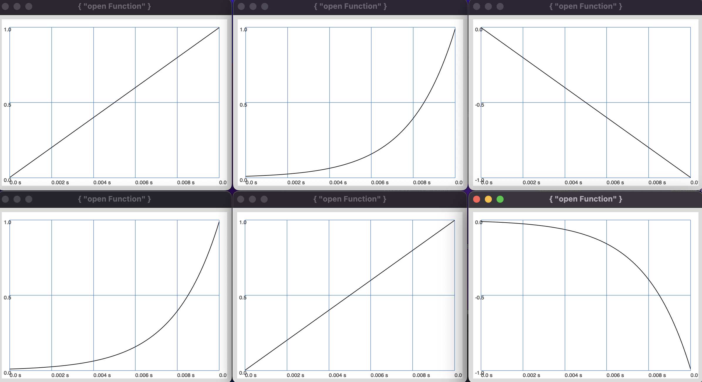
Fig. 4 The resulting plots of the code above.#
lincurve and curvelin give us a little bit more control over the shape of the transformation.
A positive curve value results in a convex, a negative value in a concave function.
(
var dur = 0.01;
{Line.ar(dur: dur).lincurve(
  inMin: 0, inMax: 1, outMin: 0, outMax: 1, curve: 1)}.plot(dur);
{Line.ar(dur: dur).lincurve(
  inMin: 0, inMax: 1, outMin: 0, outMax: 1, curve: 5)}.plot(dur);
{Line.ar(dur: dur).lincurve(
  inMin: 0, inMax: 1, outMin: 0, outMax: 1, curve: -5)}.plot(dur);

{XLine.ar(0.01, 1, dur).curvelin(
  inMin: 0.01, inMax: 1, outMin: 0, outMax: 1, curve: 1)}.plot(dur);
{XLine.ar(0.01, 1, dur).curvelin(
  inMin: 0.01, inMax: 1, outMin: 0, outMax: 1, curve: 10)}.plot(dur);
{XLine.ar(0.01, 1, dur).curvelin(
  inMin: 0.01, inMax: 1, outMin: 0, outMax: 1, curve: -5)}.plot(dur);
)
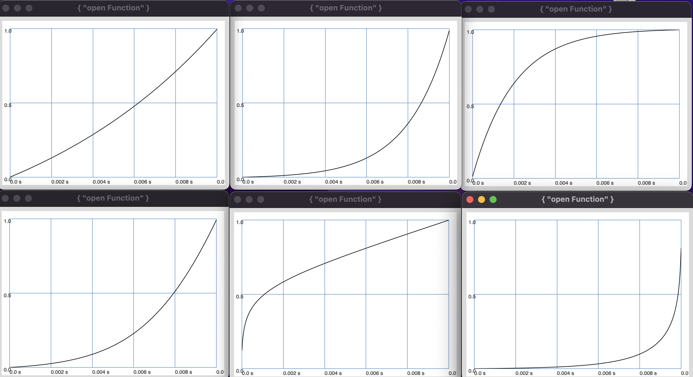
Fig. 5 The resulting plots of the code above.#
Two functions which are very helpful to change the range of a unit generator are range and bipolar.
range expects two values min and max while bipolar is a shorthand for range(a, -a).
For example, the following code posts values in \([100;400]\) to the post window.
{SinOsc.ar(1).range(100, 400).poll}.play
Random Sampling#
sclang offers many useful functions to generate pseudorandom values.
This is especially useful in the domain of algorithmic composition, since variations comes often not from human input but random variables.
For example, if we want to generate random midi notes but we want to use much more low notes than high ones we could use exprand.
{exprand(40, 80).floor}!10
Another neat function to use is nearestInScale which transforms a number to the nearest number in a specific scale.
For example, the following code gives us midi notes which belong to the C major scale.
{exprand(36, 59).nearestInScale(Scale.major)}!10
We need the brackets to evaluate the function multiple times.
The following build-in sampling functions can be used, where the receiver x is a number:
coin(x): returnstruewith the probability ofxandfalsewith the probabilityx-1.rand(x): uniformly distributed number from0up tox(exclusive).rand2(x): uniformly distributed number from-xup tox.rrand(a, b): a random number in the interval ]a,b[.linrand(x): a linearly distributed random number from zero tox.bilinrand(x): a bilateral linearly distributed random number from-xtox.sum3rand(x): a random number from-xtoxis the result of summing three uniform random generators to yield a bell-like distribution.gauss(x, sigma): a gaussian distributed random number with the standard deviationsigma.exprand(a, b): an exponentially distributed random number in the interval ]a,b[.
The following code generates histograms for some of the random generators.
(
~histogram = {
  arg values, steps = 500;
  var histogram;
  histogram = values.histo(steps: steps).normalizeSum;
  histogram;
};

~histogram.( values: {rand(4.0)}!1000000, steps: 100 ).plot(name: "uniform");
~histogram.( values: {linrand(4.0)}!1000000, steps: 100 ).plot(name: "linear");
~histogram.( values: {bilinrand(4.0)}!1000000, steps: 100 ).plot(name: "bilinear");
~histogram.( values: {sum3rand(4.0)}!1000000, steps: 100 ).plot(name: "pseudo gauss");
~histogram.( values: {gauss(0.0, standardDeviation: 1.0)}!1000000, steps: 100 ).plot(name: "gauss");
~histogram.( values: {exprand(4.0, 0.5)}!1000000, steps: 100 ).plot(name: "exp");
)
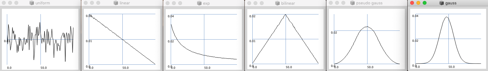
Fig. 6 Plot of a histogram of rand(x), linrand(x), exprand(a, b), bilinrand(x), sum3rand(x), gauss(x, sigma).#
On the server-side there are corresponding unit generators such as
Signal Lagging#
We are sometimes in a situation where we want to change the output of a signal from one value to another but we desire a smooth transition, e.g., to avoid clicks.
Lagging a signal via the lag function filters the signal via a lowpass filter such that a smooth transition is accomplished.
Instead of dealing with abstract filter arguments, it lets you conveniently define the duration of the transition.
It is equivalent to the Lag unit generator.
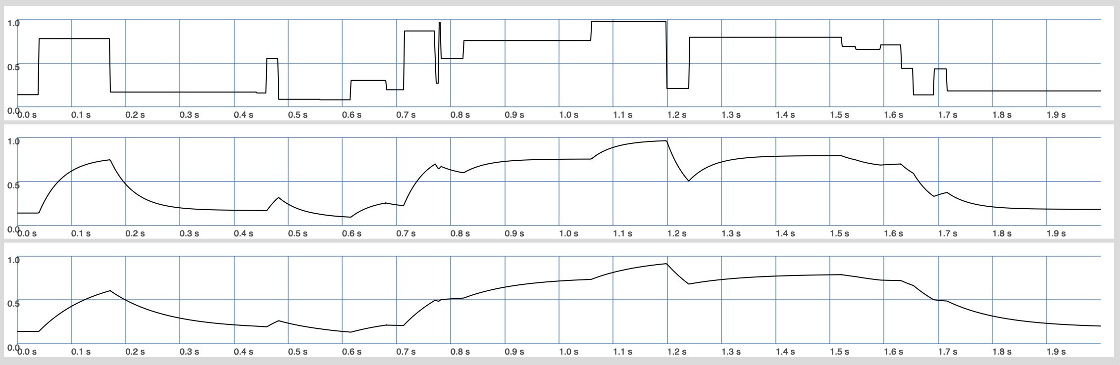
In the following we use the TRand unit generator triggered by a Dust ugen to spill out the same random number over a short duration, determined by the next trigger signal. The plot below shows the unfiltered signal and two filtered signals with different lag times.
({
  var sig = TRand.ar(0, 1, Dust.ar(10));
  sig = [sig, sig.lag(0.3), sig.lag(0.7)]
}.plot(2);
)
Debugging#
Sometimes we want to know what stream or flow of numbers we generate.
To post the numbers a unit generator produces to the post window you can use poll.
For patterns and other language/client side functions you can use trace instead.
Examples#
In the following example we use frequency for \freq, amplitude for \amp and semitones for \detune.
Furthermore, we convert -7 decibels into amplitude and make use of k.reciprocal which computes 1/k.
The sound is generated by three sine waves at frequency \freq, \freq + 0.01 semitones and \freq - 0.01 semitones.
Since the detuning is very small we can hear the sine wave going in and out of phase.
(
SynthDef(\detune_sines, {
    arg freq=440, detune=0.2, amp = 0.5;
    var sig, env;
    sig = SinOsc.ar(freq * [0.0, detune, (-1)*detune].midiratio);
    sig = sig * amp * 3.reciprocal;
    sig = Splay.ar(sig);
    Out.ar(0, sig);
}).add;
)

Synth(\detune_sines, [\freq, 440, \amp, -7.dbamp, \detune: 0.01]);
Let us look at another example using patterns.
(
SynthDef(\blip,{
  arg freq = 440, amp = 0.5, atk = 0.01, rel = 0.3, detune = 0.1;
  var sig, env;

  sig = Pulse.ar(freq * [0.0, detune, (-1)*detune].midiratio);
  env = Env.perc(atk, rel).ar(doneAction: Done.freeSelf);
  sig = sig * env * amp;
  sig = Mix(sig);
  Out.ar(0, sig!2);
}).add;

)

(
Pbind(
  \instrument, \blip,
  \scale, Scale.minor,
  \root, 1,
  \degree, Pfunc({gauss(0, 5).floor}),
  \rel, Pkey(\degree).linexp(inMin: -7, inMax: 7, outMin: 0.5, outMax: 0.1),
  \octave, Prand([6,6,6,6,7], inf),
  \dur, 1/8,
  \detune, Pseries(0, 0.01, 200)
).play
)
First, I define a basic synth definition that generates a percussive pulse computer-game-like sound.
Again, I use the detuning technique.
Then I play an event pattern using the defined synth \blip.
I play in the scale of D minor using a gaussian distribution around the tonic.
Furthermore, I modulate the release time with respect to the degree of the note such that high-degree notes have an exponentially shorter release time!
Thereby, I mimic the natural effect of faster disappearing high frequencies.
In addition, the \detune increases from 0 to 0.01 times 200.
Let us use two sine waves changing their frequency 5 times a second via a smooth transition. To achieve the rate of change we use the Impulse ugen:
{0.25 * SinOsc.ar(TRand.ar(200, 1000, Impulse.ar(5)!2).lag(0.3))}.play