Basic Filters

Most filters you will encounter are linear as well as time-invariant (by default if we do not modulate their arguments), and the best way to understand them is by either using them or by looking at their frequency and impulse responses, see section LTI Filters.

We usually do not use the following two filters since their arguments are sample rate dependent. Instead, we rely on filters for which we can define more meaningful arguments, such as a cutoff frequency. However, these more convenient filters are based on more low-level filters, such as the following ones. So let’s have a look.

OneZero

We have already analyzed one of the most simple filters called one zero filter. The unit generator OneZero realizes such a filter. It extends the Filter class and is a linear time-invariant filters. It is not trivial to see what is happening if we only look at the implemented formula:

\[y[n] = (1 - |\alpha|) \cdot x[n] + \alpha \cdot x[n-1], \quad -1 \leq \alpha \leq 1\]

For \(\alpha < 0\) OneZero is a highpass filter and for \(\alpha > 0\) it is a lowpass filter.

OneZero

For \(\alpha > 0\) OneZero is a lowpass filter and for \(\alpha < 0\) it is a highpass filter.

If we apply the filter to a signal \(x\) that has a constant difference quotient, all values of the output \(y\) are almost zero. This can be demonstrated by using a sawtooth wave. We can use the OneZero-filter to achieve this effect.

{[LFSaw.ar(10), OneZero.ar(LFSaw.ar(10), -0.5)]}.plot(2/10)

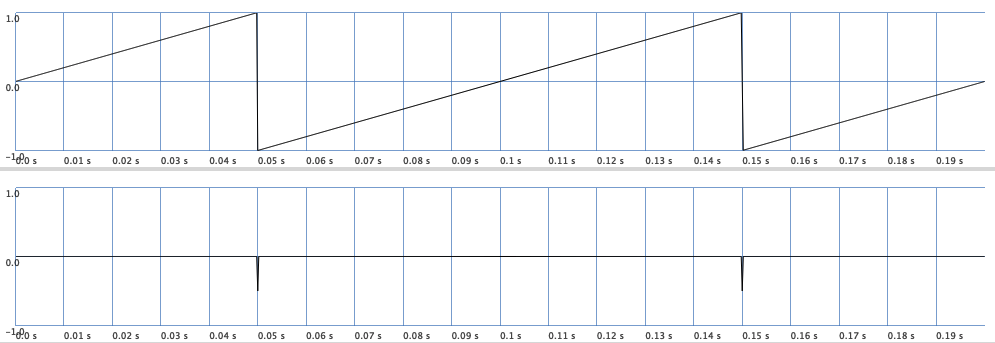
Fig. 49 Canceling a sawtooth wave by applying a OneZero-filter. You can see peaks at values where the sawtooth is not differentiable.

This cancelation works so well because the rate of change of a sawtooth wave is constant almost everywhere.

Without using the Z-transform, I had a hard time understanding what this filter actually does to its input signal \(x\), since the documentation is very minimal. But let us think about the formula a little bit without going into the theory of filters.

It is important to note that \(x[n]\) is the \(n\)-th sample of the discrete input signal. Therefore, OneZero-filter (as well as OnePole) depend on the sample rate or sample frequency \(f_s\)! Using \(\alpha = -0.5\) gives us almost the difference quotient

\[y[n] = 0.5 \cdot x[n] - 0.5 \cdot x[n-1].\]

In other words, we get

(66)\[\begin{equation} \frac{x(t) - x(t - \Delta t)}{2\Delta t}, \end{equation}\]

where \(\Delta t\) is \(f_s^{-1}\) seconds. To get the difference quotient, we have to multiply by a factor of two.

To test this result, let us compute the cosine using SinOsc and a OneZero. Remember

(67)\[\begin{equation} \frac{d\sin(2\pi \cdot \omega \cdot t)}{dt} = 2 \pi \cdot \omega \cdot \cos(2\pi \cdot \omega \cdot t) \end{equation}\]

({
    var freq = 220;
    var sample_rate = 48000;
    var dt = sample_rate.reciprocal;

    [
        OneZero.ar(SinOsc.ar(freq), -0.5) * 2 / dt / (2 * pi * freq), 
        SinOsc.ar(freq)
    ]
}.plot(1/220)
)

The following plot reveals this relationship.

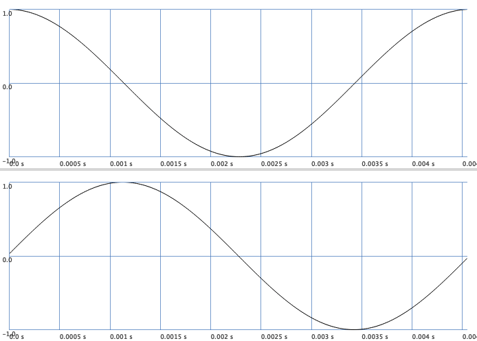
Fig. 50 At the top, the cosine is generated by the bottom signal and a OneZero unit generator.

Slope UGen

The Slope unit generator can also be used to compute the slope of a signal.

Slope.ar(SinOsc.ar(freq)) / (2 * pi * freq);

gives us the cosine.

For \(\alpha = 1.0\), we delay the signal by a single sample, and for -1.0, we additionally mirror the signal at the \(x\)-axis. For a more in-depth analysis of the frequency response, visit section Analysis of a Simple Filter.

OnePole

Another unit genertor I had a hard time get my head around is OnePole. Again let us try our best to understand what is going on without using the Z-transform.

The documentation states that a one pole filter implements the formula:

(68)\[y[n] = (1 - |\alpha|) \cdot x[n] + \alpha \cdot y[n-1]\]

with \(-1 \leq \alpha \leq 1\). I assume

(69)\[\begin{equation} y[0] = (1 - |\alpha|) \cdot x[0] \end{equation}\]

holds. \(y\) is the resulting signal and \(x\) the input signal of OnePole. Let us assume \(1 \geq \alpha \geq 0\), then we can rearrange Eq. (68):

(70)\[ y[n] = x[n] + \alpha \cdot (y[n-1] - x[n])\]

or

(71)\[ y[i] = y[i-1] + \beta \cdot (x[i] - y[i-1])\]

with \(\beta = 1-\alpha\). If \(\beta\) is small, (\(\alpha\) is large respectively), then output samples \(y[0], \ldots y[n]\) respond more slowly to a change in the input samples \(x[0], \ldots x[n]\). For example,

(72)\[\begin{equation} \begin{split} y[2] & = y[1] + \beta \cdot (x[2] - y[1]) \\ & = x[2] \cdot \beta + x[1] \cdot (\beta - \beta^2) + x[0] \cdot (\beta - 2\beta^2 + \beta^3)\\ & = \beta \cdot (x[2] + x[1] \cdot (1 - \beta) + x[0] \cdot (1 - \beta)^2) \\ & = (1-\alpha) \cdot (x[2] + x[1] \cdot \alpha + x[0] \cdot \alpha^2) \end{split} \end{equation}\]

and in general we get

(73)\[\begin{equation} \begin{split} y[i] = (1-\alpha) \cdot \sum\limits_{k=0}^{i} \alpha^{i-k} \cdot x[k]. \end{split} \end{equation}\]

The change from one filter output to the next is proportional to the difference between the previous output and the next input. Therefore, the signal is smoothen exponentially, which matches the exponential decay seen in the continuous-time system. The exponential decay is depicted in the plot in section One Pole Filter (Analysis).

OnePole

For \(\alpha > 0\) the OnePole is a lowpass filter and for \(\alpha < 0\) it is a highpass filter.

Compare, for example, the following similar sounding signals of a sawtooth wave, first filtered by the lowpass filter LPF and then filtered by OnePole using a large \(\alpha\):

{LPF.ar(Saw.ar(440), 400) * 0.25;}.play

{OnePole.ar(Saw.ar(440), coef: 0.98) * 0.25;}.play

A one pole filter simulates a simple (analog/electrical) RC-filter (resistance, capacity). In the Wikipedia article about lowpass filters, you can find some additional explanations regarding the relationship between the continuous electrical and discrete digital filter.