z-Transform

One important mathematical concept for understanding and designing filters is the \(z\)-transform. It is a mathematical tool used in digital signal processing (DSP) to converts a discrete-time signal, which is a sequence of real or complex numbers, into a complex frequency-domain (\(z\)-domain or \(z\)-plane) representation.

It generalizes the Fourier transform and the Laplace transform for discrete-time signals. In fact, it can be considered as a discrete-time equivalent of the Laplace transform and is a generalization of the discrete-time Fourier transform (DTFT) (not to be confused with the discrete Fourier transform), see Difference between DFT and DTFT.

(Unilateral) \(z\)-Transform

For a discrete-time signal \(x[n]\) the (unilateral) \(z\)-transform of \(x[n]\) is the formal power series

\[\mathcal{Z}\{x\} = X(z) = \sum\limits_{n=0}^\infty x[n] z^{-n},\]

where \(n \in \mathbb{Z}\) and \(z \in \mathbb{C}\) is a complex number. \(z\) is often written as \(z = re^{i\omega}\) (magnitude \(r\) and angle \(\omega\)). This version is used in cases wher \(x[n]\) is defined only for \(n \geq 0\).

In signal processing, this definition can be used to evaluate the unilateral \(z\)-transform of the unit impulse response of a discrete-time causal system.

(Bilateral) \(z\)-Transform

For a discrete-time signal \(x[n]\) the (bilateral) \(z\)-transform of \(x[n]\) is the formal power series

\[\mathcal{Z}\{x\} = X(z) = \sum\limits_{n=-\infty}^\infty x[n] z^{-n},\]

where \(n \in \mathbb{N}_0\) and \(z \in \mathbb{C}\) is a complex number. \(z\) is often written as \(z = re^{i\omega}\) (magnitude \(r\) and angle \(\omega\)).

The \(z\)-transform is central to understanding how filters and systems behave with these signals:

• System analysis: Linear time-variant filters (LTI) (EQ, reverb, compressor, etc.) can be described by a difference equation. The \(z\)-Transform lets us analyze these systems easily.

• Frequency response: By evaluating \(X(z)\) on the unit circle (\(z = e^{i\omega}\)), we recover the discrete-time Fourier transform (DTFT), which directly relates to how a filter affects different audio frequencies.

• Stability: In audio, unstable filters can cause distortion or infinite feedback. The \(z\)-transform helps determine if a system is stable by checking whether the poles lie inside the unit circle.

• Filter design: Many audio filters (FIR, IIR, biquads) are designed using \(z\)-transforms to shape frequency response.

\(X(z)\) is a complex-valued function of complex-valued \(z\). Furthermore, \(X(z)\) is defined on the \(z\)-plane while the DTFT is defined only on the unit circle, i.e, for \(|z| = 1\), that is, \(z = e^{i \omega}\). Remeber, for

\[-\pi < \omega < \pi\]

\(z = e^{i \omega}\) goes once around the unit circle.

Example in Audio

Suppose you want to design a simple echo effect:

\[y[n] = x[n] + 0.7y[n-1].\]

This recursive equation says: each output is the input \(x[n]\) plus a decayed version of the previous output \(y[n-1]\). So there is a feedback, i.e. a recurrence relation—typical for recursive (IIR) filters. Taking the \(z\)-transform gives us:

(38)\[\begin{split}\mathcal{Z}\{y[n]\} &= \mathcal{Z}\{x[n]\} + 0.7 \cdot \mathcal{Z}\{y[n-1]\} = \\ Y(z) &= X(z) + 0.7 \cdot z^{-1} Y(z).\end{split}\]

Here, we make use of the following property (for causal signals starting at \(n \geq 0\))

\[\mathcal{Z}\{y[n-k]\} = z^{-k}Y(z).\]

We can show this the following way:

\[\begin{split} \mathcal{Z}\{y[n-k]\} &= \sum_{n=k}^\infty y[n-k] z^{-n}\\ &= \sum_{m=0}^\infty y[m] z^{-(m+k)} \quad \text{ we define $m:= n-k \Rightarrow n = m+k$}\\ &= \sum_{m=0}^\infty y[m] z^{-m}z^{-k} = z^{-k} \sum_{m=0}^\infty y[m]z^{-m} = z^{-k}\mathcal{Z}\{y[n]\} \end{split}\]

\(z\)-tranform of Delayed Signal

Let \(y\) be a discrete-time signal then

(39)\[\begin{equation} \mathcal{Z}\{y[n-k]\} = z^{-k}\mathcal{Z}\{y[n]\} \end{equation}\]

holds.

Now we can rearranging Eq. (38) to get

\[H(z) = \frac{Y(z)}{X(z)} = \frac{1}{1-0.7z^{-1}}.\]

• \(H(z)\) is the transfer function of the filter.

• Poles at \(z = 0.7\), which is inside the unit circle \(\Rightarrow\) stable.

• On the unit circle, \(H(e^{i\omega})\) tells us how different frequencies are amplified or attenuated.

Remeber that \(z = a + bi\) with \(a,b \in \mathbb{R}\) represents a sinosoid \(r \cdot (\cos(\phi) + i\sin(\phi))\) with \(r^2 = a^2 + b^2\) and \(\phi = \cos^{-1}(a/r)\) and that the product of two complex numbers is the product of their magnitudes and the sum of their angles (see section Complex Numbers). Therefore, multiplying a sinosoid by

\[e^{-i\omega} = \cos(\omega) + i\sin(\omega) = a + bi\]

is equivalent to shift the sinosoid by \(\omega\).

This analysis is exactly how digital reverbs, delays, and EQs are studied in practice. If we delay the signal \(y[n]\) by 1 sample, \(y[n-1]\) is literally the shifted waveform (shifted to the right). In DSP, “delay by 1 sample” is like passing the signal through a one-sample delay box/system. This delay shows up as \(z^{-1}\) in the \(z\)-transform.

Each time we delay by 1 sample, the transform gets multipield by \(z^{-1}\). On the unit cirlce, \(z\) is equal to \(e^{i\omega}\) thus one delay is equivalent to multiply by \(e^{-i\omega}\) (\(\omega = 2\pi f / f_s\), where \(f\) is the real-world frequency of a sinosoid in Hz, \(f_s\) the sampling frequency in Hz and \(\omega\) the corresponding digital frequency in radians/sample). The delay shifts the phase of every frequency component by \(-\omega\) radians per delay step.

• Low frequencies (small \(\omega\)) lead to small phase shifts.

• High frequencies (large \(\omega\)) lead to big phase shifts.

That’s why in filters made of delays (echo, comb filter, reverb), frequencies interfere differently: some cancel, some reinforce! This behaviour gives us the EQ-like “tone color” of those effects.

Intuition for Audio

In time-domain, audio is just a stream of samples \(\{x[0], x[1], x[2], \ldots \}\). In frequency-domain, audio is a mix of sinusoids (cf. section Discrete Fourier Transform). The \(z\)-transform is like a superset: it captures both the frequency content and the dynamics of filters.

In fact, in audio, everything is built from delays:

• Reverb? A whole forest of delays.

• Echo? A few long delays.

• EQ filter? A mix of short delays with feedback.

In the \(z\)-domain:

• Each unit delay becomes a factor of \(z^{-1}\)

• A system made of multiple delays becomes a polynomial in \(z^{-1}\)

This is why filter transfer functions look like:

\[H(z) = \frac{b_0 + b_1 z^{-1} + b_2 z^{-2} + \ldots }{1 + a_1 + z^{-1} + a_2 z^{-2} + \ldots }\]

(top = feedforward delays, bottom = feedback delays).

By analyzing \(H(z)\) we get the most important information: Zeros i.e (roots of numerator) kill/cancel frequencies near their angle on the unit circle. Poles, i.e. (roots of denominator) boost frequencies near their angle (resonances). And the closer a pole/zero is to the unit circle, the stronger its effect.

The unit circle is acts as the frequency axis. Therefore, \(H(z)\) evaluated on the unit circle, i.e. \(z = e^{i\omega}\) and sweeping \(\omega\) from \(0\) to \(\pi\) literally sweeps from \(0\) to Nyquist and the magnitude \(|H(e^{i\omega})|\) tells us gain at that frequency. This is how the \(z\)-transform connects directly to what our ears hear.

Furthermore, in audio feedback is everywhere (delays, reverb, resonant filters).

• If a pole is inside the unit circle \(\Rightarrow\) energy decays \(\Rightarrow\) stable reverb/echo.

• If a pole is outside \(\Rightarrow\) energy grows \(\Rightarrow\) runaway feedback (squeal!).

So the \(z\)-transform is the natural tool to reason about when feedback produces musical resonance vs. disaster.

Overall we can think of the \(z\)-transform as a map of how sound flows through delays and feedback:

• Time-domain: “What is the output sample right now?”

• Frequency-domain: “Which tones are emphasized or reduced?”

• \(z\)-domain: “How do delays + feedback combine to shape all tones over time?”

It’s the unifying lens that lets audio engineers go from “this is the equation of my filter” to “this is how it colors the sound”.

Region of Convergence

The region of convergence ROC is one of the most important (and sometimes confusing) aspects of the \(z\)-transform. Let’s break it down carefully in the context of audio/DSP.

When you define the z-transform

\[X(z) = \sum\limits_{n=0}^\infty x[n] z^{-n},\]

that series may or may not converge depending on the value of \(z\). The ROC is the set of \(z\) values (in the complex plane) for which that infinite sum converges. If it does not converge, the \(z\)-transform of the signal does not exist (for that \(z\)).

Example 1

For example, let us look at a delayed impulse \(x[n] = \delta[n-n_0]\) with \(n \geq n_0\). Here \(\delta\) is the Kronecker \(\delta\)-function. We get

\[\mathcal{Z}\{\delta[n-n_0]\} = \sum\limits_{n=0}^\infty \delta[n-n_0] z^{-n} = z^{-n_0} = \frac{1}{z^{n_0}}\]

which does not converge for \(z = 0\) because it blows up (\(1/z^{n_0} \rightarrow \infty\) for \(z \rightarrow 0\)).

Example 2

Let us look at another example: an exponential decay

\[x[n] = \alpha^n \cdot u[n] = \alpha^n \cdot 1 = \alpha^n.\]

In this case, we get

(40)\[\begin{equation} \begin{split} X(z) &= \sum\limits_{n = 0}^\infty x[n] z^{-n} = \sum\limits_{n = 0}^\infty \alpha^n z^{-n}\\ &= \sum\limits_{n = 0}^\infty (\alpha z^{-1})^n. \end{split} \end{equation}\]

Since this is a geometric series, this gives us a nice closed-expression

\[X(z) = \frac{1}{1-\alpha z^{-1}},\]

if \(|\alpha z^{-1}| < 1\), otherwise \(X(z)\) does not converge. Note that we need either the series expansions or the ROC plus the closed-expression to know everything because

\[\frac{1}{1-r} = +\sum_{n=0}^\infty r^{+n}, \quad |r| < 1\]

and

\[\frac{1}{1-r} = -\sum_{n=0}^\infty r^{-n}, \quad |r| > 1\]

is true.

General Properties

First, if \(x[n]\) is a finite duration signal, then the ROC contains all \(z\) except possibly \(z=0\) and \(z = \infty\). In this case the \(z\)-transform is just a finite polynomial in \(z^{-1}\):

\[X(z) = \sum_{n=n_1}^{n_2} x[n] z^{-n}\]

and this finite sum converges for all \(z \in \mathbb{C}\), except at \(z=0\) if the signal has nonzero positive-time samples or \(z = \infty\) if the signal has nonzero negative-time samples. Note that the system’s/filter’s impulse response can be infinite in duration in audio processing (e.g., reverb tail, recursive filter).

Second, the region of convergence (ROC) is either the region

1. inside a circle (\(|z| < r_L\)),

2. outside a circle (\(|z| > r_R\)) or

3. a ring (\(r_R < |z| < r_L\)).

Third, the ROC can not contain any poles.

An LTI filter/system is BIBO stable if the unit circle (\(|z| = 1\)) is inside the ROC (the ROC includes \(|z| = 1\) if and only if the discrete-time Fourier transform (DTFT) exists). In audio: stability means

finite input leads to finite output.

If the ROC does not include \(|z| = 1\), the system is unstable (runaway feedback) and only if it is included, we are able to compute a valid frequency response. If not then the system has no well-defined steady-state frequency response.

For LTI filter/system, if the impulse response’s ROC extends outward from the outermost pole (i.e. \(|z| > |p_{\text{max}}|\)), the system is causal. In audio: causal systems mean

no response before the input occurs \(\Rightarrow\) physically realizable filter.

In summary, the shape of the ROC encodes causality and stability, while the position of poles/zeros encodes tone color (resonance, notches).

Poles and Zeros

Most useful and important \(z\)-transforms are those who give us rational functions

\[X(z) = \frac{P(z)}{Q(z)},\]

with \(P(z), Q(z)\) to be polynomials in \(z\). The zeros are values of \(z\) for which \(X(z) = 0\) and the poles are values of \(z\) for which \(X(z) = \infty\). The roots of \(P(z)\) are the zeros and the roots of \(Q(z)\) are the poles. (\(X(z)\) may also have poles/zeros at \(z = \infty\), if the order of the two polynomials differ.)

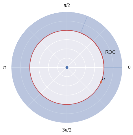
Example 1

Let us look at the following signal—a repeated but decaying impulse:

\[x[n] = \alpha^n u[n] = \alpha^n, \quad \forall n \in \mathbb{N}_0: u[n] = 1.\]

Let us compute the \(z-\)transform of this signal:

\[\mathcal{Z}\{\alpha^n u[n]\} = X(z) = \sum_{n=0}^\infty \alpha^n z^{-n} = \sum_{n=0}^\infty \left(\frac{\alpha}{z}\right)^n = \frac{z}{z-\alpha}, \quad \text{ if } |z| > |\alpha|.\]

In this case there is a pole at \(z = \alpha\) and a zero at \(z = 0\). The following plot shows zeros in blue and poles in orange. The region of convergence (ROC) (in blue) is outside of the (red) circle of radius \(\alpha\). It extends outwards from the outermost pole thus the system is causal.

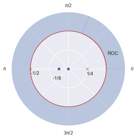
Example 2

Let us look at another example:

\[\mathcal{Z}\left\{ \left( \frac{1}{4} \right) u[n] + \left( \frac{-1}{2}\right)^n u[n]\right\} = X(z) = \frac{z}{z-1/4} + \frac{z}{z + 1/2}, \quad |z| > 1/2\]

Using some algebra, we get

\[X(z) = \frac{z^2 + 1/2 z + z^2 - 1/4 z}{(z-1/4)(z+1/2)} = \frac{2z(z+1/8)}{(z-1/4)(z+1/2)}, \quad |z| > 1/2\]

All zeros (\(z = 0\), \(z = -1/8\)) and poles (\(z = 1/4\), \(z = -1/2\)) are on the real-axis. Again the ROC extends outwards from the outermost pole thus the system is causal.

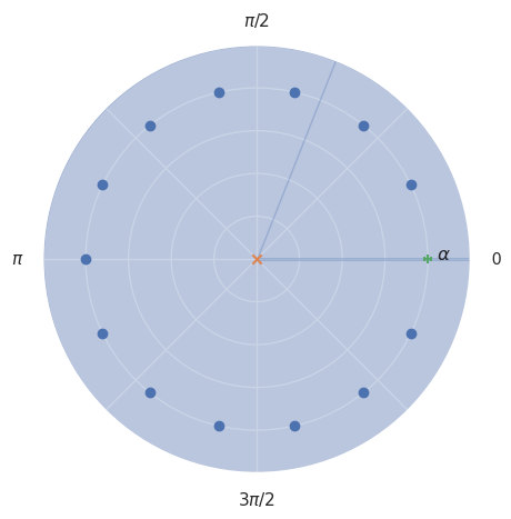
Example 3

Let us look at another example were

\[\begin{split} x[n] = \begin{cases} \alpha^n, & \text{ if } 0 \leq n \leq N-1\\ 0, & \text{ otherwise}. \end{cases} \end{split}\]

Then,

\[X(z) = \sum\limits_{n=0}^{N-1} (\alpha z^{-1})^n.\]

This is a geometric series thus

\[X(z) = \frac{1 - (\alpha z^{-1})^N}{1 - \alpha z ^{-1}} = \frac{z^N- \alpha^N}{z^{N-1}(z-\alpha)}.\]

This geometric series converges for \(|\alpha| < \infty\) and \(z \neq 0\). Therefore, the ROC is the entire \(z\)-plane, except \(z = 0\). Our single pole is at \(z = 0\) since \(z = \alpha\) cancels out with our zero \(z_0 = \alpha\). Remeber that when we multiply a complex number by another complex number, the result is another complex number that is a rotated and scaled version of the first one. The equation \(z^N = \alpha^N\) should have \(N\) solutions. De Moivre’s theorem states that for \(z = r \cdot e^{i \phi}\)

\[z^N = r^N \cdot \underbrace{e^{i \cdot n \cdot \phi}}_{\text{rotation}}.\]

If we set \(r = \alpha\) we get

\[z^N = r^N \cdot e^{i \cdot N \cdot \phi} = \alpha^N \cdot e^{i \cdot N \cdot \phi} = \alpha^N.\]

Note that \(|e^{i \cdot N \cdot \phi}| = 1\). So we search angles \(\phi_k\) such that rotating \(\alpha^N\) \(n\)-times with angle \(\phi_k\) gives us \(\alpha^N\). If we rotate by 360 degrees, i.e. \(2\pi\) we clearly land on \(\alpha^N\)! Therefore,

\[\phi_k = \frac{2\pi}{N} \cdot k, \quad k = 1, 2, 3, \ldots, N-1.\]

Thus our zeros are

\[z_k = \alpha \cdot e^{i \frac{2\pi}{N} k}, \quad k = 1, 2, 3, \ldots, N-1.\]

The following plot shows poles and zeros for some \(\alpha \in \mathbb{R}^+\).

In general, if \(X(z) = \frac{P(z)}{Q(z)}\) and the order of \(P(z)\) is \(M\) while the order of \(Q(z)\) is \(N\) then:

1. \(N > M \Rightarrow N-M\) zeros at \(z = \infty\)

2. \(M > N \Rightarrow M-N\) poles at \(z = \infty\).

Power Series Expansion

The power series expansion is how the abstract algebraic fraction \(H(z)\) is translated back into a sequence of samples (impulse response).

\[X(z) = \sum\limits_{n=0}^\infty x[n] z^{-n}\]

is itself a power series. Therefore, what we have to do is, to identify \(x[n]\) as coefficient of \(z^{-n}\). For example, given

\[X(z) = 1 + 3z^{-1} - 4z^{-4}\]

we can write this like

\[X(z) = x[0] z^0 + x[1] z^{-1} - x[4] z^{-4},\]

thus

\[x[n] = \delta[n] + 3 \delta[n-1] - 4 \delta[n-4]\]

where \(\delta\) is the Kronecker \(\delta\)-function.

We can also invert rational \(X(z)\) with long division. Let us assume

\[X(z) = \frac{1-z^{-1}}{1-1/2 z^{-1}}\]

is given. For the ROC \(|z| > 1/2\) has to hold.

Now we can just compute \((1-z^{-1}) / (1-1/2 z^{-1})\) which gives us

\[1 - 1/2 z^{-1} - 1/4 z^{-2} - 1/8 z^{-3} - 1/16 z ^{-4} - \ldots\]

thus

\[x[n] = 2\delta[0] -\left( \frac{1}{2} \right)^n u[n].\]

Partial Fraction Expansion

Given a rational function in the \(z\)-domain, which typically represents a system’s transfer function or a signal’s \(z\)-transform, the goal is to express it as a sum of simpler fractions, that is as partial fraction expension (PFE), because:

• Easier inverse \(z\)-transform: Instead of trying to invert a complicated rational function, you invert each simple term individually.

• Clear connection to poles/resonances: Each term in the PFE corresponds to one pole, i.e. one resonant component in the sound.

• Intuitive analysis of system behavior: If you know the poles and residues (\(A_i\)), you can immediately tell if the system is causal or anti-causal from the ROC. Furthermore, you can see which components dominate (e.g. the pole closest to the unit circle sets the longest-lasting resonance).

• Practical for implementation: In DSP, many filters (like IIR biquads) are implemented as a sum of simple sections. Therefore, PFE naturally decomposes a high-order filter into first- or second-order pieces, each easy to implement with delay lines. This makes designs stable and efficient.

The process to compute the partial fraction expension (PFE) involves the following steps:

1. Factor the denominator: Write the denominator of the \(z\)-domain function as a product of its factors. If the factors are not real, they will appear as conjugate pairs.

2. Decompose the function: Express the original function as a sum of simpler fractions, where each fraction has one of the factors from the denominator as its own denominator. The numerators of these simpler fractions are constants or polynomials (typically constants in \(z\)-transform applications) to be determined.

3. Find the constants: Use algebraic techniques, such as equating coefficients or substituting specific values of \(z\), to solve for the constants (or coefficients in the numerators) in the simpler fractions.

4. Inverse \(z\)-transform: Apply the inverse \(z\)-transform to each simpler fraction separately. Since the inverse \(z\)-transform of many basic fractions is well-known, this step is greatly simplified by the partial fraction expansion.

The case of first-oder terms is the simplest and most fundamental, that is, we have

\[H(z) = \frac{B(z)}{A(z)} = \frac{b_0 + b_1 z^{-1} + b_2z^{-2} + \ldots + b_m z^{-M}}{1 + a_1 z^{-1} + a_2 z^{-2} + \ldots + a_N z^{-N}},\]

where \(M < N\) and we want to compute

\[H(z) = \sum\limits_{k=1}^N \frac{r_k}{1- p_k z^{-1}}.\]

\(p_k\) are the poles of the transfer function, and each numerator \(r_k\) is called residue of pole \(p_k\). Both the poles and their residues may be complex. The poles may be found by factoring the polynomial \(A(z)\) into first-order terms. The residue \(r_k\) corresponding to pole \(p_k\) may be found analytically as

\[r_k = (1- p_k z^{-1}) H(z)|_{z = p_k}\]

when the poles \(p_k\) are distinct. Thus, it is the “residue” left over after multiplying \(H(z)\) by the pole term \((1- p_k z^{-1})\) and letting \(z\) approach \(p_k\). In a partial fraction expansion, the \(k^{\text{th}}\) residue \(r_k\) can be thought of as simply the coefficient of the \(k^{\text{th}}\) one-pole term \(r_k/(1-p_k z^{-1})\) in the PFE.

Example

Consider the two-pole filter

\[H(z) = \frac{1}{(1-z^{-1}) (1- 0.5 z^{-1})}\]

The poles are \(p_1 = 1\) and \(p_2 = 0.5\). The corresponding residues are then

\[r_1 = (1-z^{-1}) H(z)|_{z=1} = \frac{1-z^{-1}}{(1-z^{-1}) (1-0.5 z^{-1})}\bigg|_{z=1} = \frac{1}{1-0.5 z^{-1}}\bigg|_{z=1} = 2\]

and

\[r_2 = (1-0.5z^{-1}) H(z)|_{z=0.5} = \frac{1-0.5z^{-1}}{(1-z^{-1}) (1-0.5 z^{-1})}\bigg|_{z=0.5} = \frac{1}{1-z^{-1}}\bigg|_{z=0.5} = -1.\]

Therefore, we can conlcude that

\[H(z) = \frac{2}{^-z^{-1}} - \frac{1}{1-0.5z^{}-1}.\]

Complex Example

Consider the filter defined by

\[H(z) = \frac{a}{1+z^{-2}}, \quad a \in \mathbb{C}.\]

The poles are \(p_1 = i\) and \(p_2 = -i\) since \(i^{-2} = (-i)^{-2} = i^{2} = 1\). Thus we can rewrite \(H(z)\) in factored form

\[H(z) = \frac{a}{(1-i z^{-1}) (1+i z^{-1})}.\]

We can use the same equation to get the residues:

\[r_1 = (1-iz^{-1}) H(z)|_{z=i} = \frac{a}{1+i z^{-1}}\bigg|_{z=i} = \frac{a}{2},\]

and

\[r_2 = (1+iz^{-1}) H(z)|_{z=-i} = \frac{a}{1-i z^{-1}}\bigg|_{z=-i} = \frac{a}{2}\]

Therefore we arrive at

\[H(z) = \frac{a/2}{1-i z^{-1}} + \frac{a/2}{1+iz^{-1}}.\]

LTI Analysis

Until now we worked with examples of a LTI filter. It is now time to generalize to any LTI filter.

The general form for a difference equation is given by (and representing a linear time-invariant filter)

(41)\[\begin{equation} \sum\limits_{k=0}^N a_k y[n-k] = \sum\limits_{k=0}^M b_k x[n-k], \quad a_0 \neq 0 \end{equation}\]

Usually \(a_0 = 1\).

Transfer Function of LTI Filters

If we take the \(z\)-transform of both sides we get:

\[\begin{equation*} \sum\limits_{k=0}^N a_k z^{-k}Y(z) = \sum\limits_{k=0}^M b_k z^{-k} X(z) \iff Y(z) \sum\limits_{k=0}^N a_k z^{-k}= X(z) \sum\limits_{k=0}^M b_k z^{-k}. \end{equation*}\]

In this step we use Eq. (39). Solving for \(Y(z)\) gives us

\[\begin{equation*} Y(z) = \underbrace{\frac{\sum\limits_{k=0}^M b_k z^{-k}}{\sum\limits_{k=0}^N a_k z^{-k}}}_{H(z)} X(z) = H(z) X(z) \end{equation*}\]

where \(H(z)\) is the transfer function.

Transfer Function of LTI Filters

The transfer function \(H : \mathbb{C} \rightarrow \mathbb{C}\) of a linear filter

(42)\[\begin{equation} \sum\limits_{k=0}^N a_k y[n-k] = \sum\limits_{k=0}^M b_k x[n-k], \quad a_0 \neq 0 \end{equation}\]

is defined by

(43)\[\begin{equation} H(z) = \frac{\sum\limits_{k=0}^M b_k z^{-k}}{\sum\limits_{k=0}^N a_k z^{-k}}. \end{equation}\]

If \(b_0 \neq 0\) then

\[\begin{equation*} H(z) = \frac{b_0}{a_0} \frac{\prod\limits_{k=1}^M (1 - c_k z^{-1})}{\prod\limits_{k=1}^N (1 - d_k z^{-1})} \end{equation*}\]

where \(c_k\) for \(k = 1, 2, \ldots M\) are zeros and \(d_k\), for \(k = 1, 2, \ldots N\) are poles.

Transfer Funktio and Impulse Response

The transfer function \(H : \mathbb{C} \rightarrow \mathbb{C}\) of a linear filter is the \(z\)-transform of the impulse response of the filter, i.e.,

(44)\[\begin{equation} H(z) = \mathcal{Z}\{h[n]\} \end{equation}\]

Example 1: Filter Equation to Transfer Function

Let use start with a very simple filter. I will re-use this example in section Analysis of a Simple Filter.

\[\begin{equation*} y[n] = x[n] + x[n-1], \quad n = 0, 1, 2, \ldots \end{equation*}\]

We have \(b_0 = b_1 = a_0 = 1\). Therfore the transfer function is determined by

\[H(z) = \frac{b_0 + b_1 z^{-1}}{a_0} = \frac{1 + z^{-1}}{1} = 1 + z^{-1}\]

Therefore, there is a zero at \(z = -1\). The frequency response of the filter is given by

\[H(e^{i\omega}) = 1 + e^{-i\omega}.\]

The following plot illustrates the behavior of \(H\). Each point on the unit circle represents a specific frequency between \(-f_s/2\) and \(f_s/2\). The gain in amplitude for such a point (frequency) is the length of the line segment of that point to the zero! I draw one such line in blue and some of the points. Imagine the grey point connected to the cross going around on the unit circle.

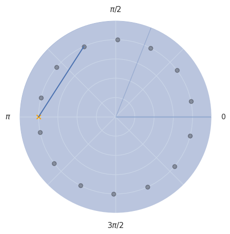
With only one zero, the effect of the filter kicks only in for high frequencies, i.e. points close to the zero.

Example 2: Transfer Function to Filter Equation

Let

\[H(z) = \frac{(z+1)^2}{(z-1/2)(z+1/4)} = \frac{z^2(1 + z^{-1})^2}{z^2(1-1/2 z^{-1}) (1+1/4 z^{-1})} = \frac{1 + 2 z^{-1} + z^{-2}}{ 1 - 1/4 z^{-1} - 1/8 z^{-2}}\]

Then \(b_0 = 1\), \(b_1 = 2\), \(b_2 = 1\) and \(a_0 = 1\), \(a_1 = -1/4\), \(a_2 = -1/8\) and we get the following equation:

\[y[n] - 1/4 \cdot y[n-1] - 1/8 \cdot y[n-2] = x[n] + 2 \cdot x[n-1] + x[n-2]\]

Thus the filter is defined by

\[y[n] = x[n] + 2 \cdot x[n-1] + x[n-2] - 1/4 \cdot y[n-1] - 1/8 \cdot y[n-2].\]