Sampling#
This section introduces sampling. It is the necessary fundament for all digital signal processing and communication. Different from music production where sampling means to reuse and tinker with a recorded audio material (and usually involves the sampling I introduce in this section), sampling here is defined as the process of measuring an analog signal at distinct and usually a finite number of points. Digital representations of analog signals offer advantages in terms of
robustness towards noise, meaning we can send more bits/s
use of flexible processing equipment, in particular the (digital) computer
more reliable processing equipment
easier to adapt complex algorithms
Sampling
Sampling is the process of measuring an analog signal at distinct and usually a finite number of points.
Notation#
I use the following well-known notation:
original analog signal \(y(t)\)
sampling frequency also called sampling rate \(f_s\)
sampling interval \(T_s\), where \(T_s = 1/f_s\)
sampled signal \(y_N[n]\), where \(y_N[n] \approx y(n \cdot T_s)\)
frequency of an analog signal \(f\)
The Process of Sampling#
On a (digital) computer we are dealing with digital signals, that is, discrete signals. There is no way around this fact. Sampling is the technique to transform a continuous function
into a discrete representation
Remember, we are interested in continuous and discrete 1D signals \(y(t)\) and \(y_N(n)\) respectively where the independent variable is time \(t\) and the timestep \(n\). So we start off with an analog signal which is then sampled uniformly! Uniform sampling implies that we sample every \(T_s\) seconds or \(f_s\) times a second.
Loss of Information#
Indeed, that’s not quite precise enough because we represent all complex number or irrational numbers by floating point numbers. Therefore, for complex a number \(z = a + ib\),
holds (most of the time). Sometimes one also wants to quantize the values of \(y_N\). Sampling in the context of audio means that we use equidistant sample points.
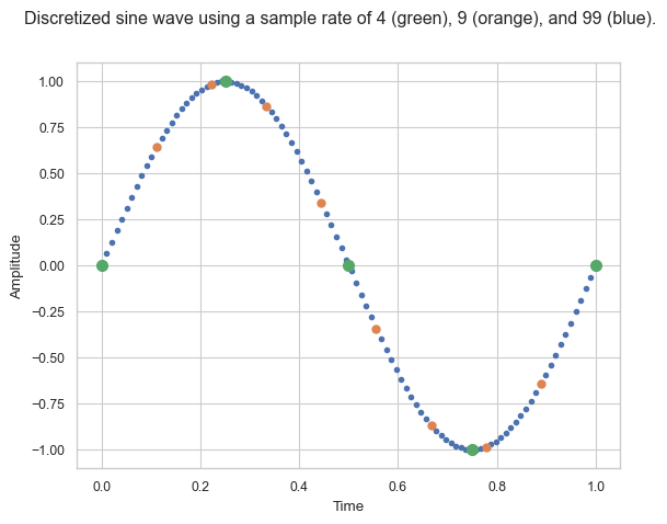
For example, let us assume our sample rate (also called sample frequency) \(f_s\) is 9 hertz (Hz), meaning we sample in an equidistant nine times a second. And let us assume we want to sample a sine wave \(y(t) = \sin(2\pi \cdot f \cdot t)\) with a frequency of 6 Hz, i.e., \(f = 1\). Then
and in general
I indicate, that the value \(y_N[n]\) is only an approximation, since on a computer we use a certain bit depth of our floating point numbers! In the image above the orange points indicate our sample points of the continuous function. You can also see that if we only use a sample rate of 2 Hz all our sample values would be zero, indicating that the sample rate is surely too small in comparison to the frequency of the sine wave.
The following code generates the samples for our example.
You can play around with the sampeRate \(f_s\) and the frequency \(f\).
Note however that the \(x\)-axis gives you the sample number (starting from 0) instead of the time \(t\).
(
var sampleRate = 4;
var frequency = 1.0;
y = {|t|
  (2*pi*frequency*t).sin;
};
Array.interpolation(sampleRate,0.0,1.0).collect({|t| y.(t)}).plot(discrete: true)
)
In summary, we lose information, i.e. accuracy on two ends: (1) first of all in the time direction but also (2) in the amplitude direction.
Aliasing#
Calling
s.sampleRate // 44100 Hz
gives us the sample rate of our audio signals.
On my machine, I use a sample rate of 44100 Hz, i.e. 44100 samples per second. Therefore, an audio signal \(y: \mathbb{N} \rightarrow \mathbb{Q}\) represents 1 second by 44100 samples (rational numbers)
If we use single-precision floating point, then each sample requires 32-bit or 4 bytes. Therefore, the signal uses up approximately 1.67 MiB (often wrongly written as MB / MegaByte). Sound in its raw form is quite memory intensive!
When the highest frequency of a signal is less than one-half of the sample rate, the resulting discrete-time sequence is said to be free of the distortion known as aliasing (different signals become indistinguishable to each other). This follows from the so called Nyquist–Shannon sampling theorem.
Nyquist–Shannon Sampling Theorem
If a function \(y(t)\) contains no frequencies higher than \(f\) hertz, it is completely determined by giving its ordinates at a series of points spaced \(1/(2f)\) seconds apart. In other words, when sampling an analog signal the sampling frequnecy must be greater than twice the highest frequency component of the analog signal to be able to reconstruct the original signal from the sampled version.
I will not prove this theorem here because it involves techniques like the Fourier transform that we have not yet covered, but from our example you get some of the intuition.
Aliasing
If the sample frequency is less than twice the highest frequency component, then frequencies in the original signal that are above half the sampling rate will be “aliased” and will appear in the resulting signal as lower frequencies.
The consequence of aliasing is that we cannot recover the original signal, so aliasing has to be avoided except if you want to use it intentionally. Sampling too slowly will produce a sequence \(y(t)\) that could have originated from a number of signals. So there is no chance of recovering the original one.
To avoid aliasing we have to sample fast enough. But if we can’t sample fast enough (possibly due to costs) we can include an anti-aliasing filter—usually a low-pass filter that is applied before sampling to ensure that no more components with frequencies greater than half the sample frequency remain. This will give us an inexact reconstruction but can still be a good enough solution.
Aliasing
Aliasing is the effect that results from a too-small sample rate by which different signals become indistinguishable from each other.
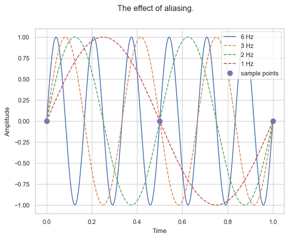
In the example above we can observe aliasing. We can see that a sample rate of 1 Hz is too low to capture \(y(t) = \sin(2\pi \cdot f \cdot t)\) for \(f = 2, 3, 6\) Hz. All these sine waves could also appear as a sine wave of 1 Hz. They are indistinguishable if we use a sample rate that low.
The human ear is able to recognize frequencies up to round about 20000 Hz. Since we need double the sample rate, 44100 gives us a little bit of room.
You can play around with the following code to see the effect of a sample rate that is too low.
Change sampleRate and re-evaluate the code.
The first plot shows a good approximation of the real signal.
The second plot shows the result of the sampling process.
(
var sampleRate = 8.0;
var frequency = 6.0;
y = {|t|
	(2*pi*frequency*t).sin;
};
[
	Array.interpolation(10000,0.0,1.0).collect({|t| y.(t)}),
	Array.interpolation(sampleRate,0.0,1.0).collect({|t| y.(t)})
].plot(discrete:false)
)